
AN INTRODUCTION
TO USING MATLAB
Eric Peasley, Department of Engineering Science, University of Oxford
version 7.1, 2019
[
1 5 7 8.8 7.42
4.6 72 5i 92 44
7i 65 77 63 4.2
3
5i 22 4.11 54 54
17.3 111 32 21 21
83.2 230 12 4i 16
]
plot(x,y,'rx')
x = linspace(-2*pi,2*pi,100)
X = [1 2 3; 4 5 6; 7 8 9]
hold on;
blank = ones(3,4)
p = polyfit(x,y,1)
y = a*x.^2 + b*x + c
D = sqrt(A)
help average
While (err>0.001)
y = 0:5:20
L = (B>=13)
whos
for k = [ 1 5 7 pi Nan inf]
title('My graph')
a = [ exp(0) sqrt(4) 1+2 ]
AN INTRODUCTION
TO USING MATLAB
Eric Peasley, Department of Engineering Science, University of Oxford
MATLAB is a registered Trade Mark of MathWorks Inc.
Version 7.1, 2019
1
2
Table of Contents
INTRODUCTION ..................................................................................................................5
STARTING MATLAB............................................................................................................6
SIMPLE EXPRESSIONS......................................................................................................7
ASSIGNMENTS....................................................................................................................8
MATHEMATICAL FUNCTIONS ..........................................................................................9
SPECIAL NUMBER SYMBOLS.........................................................................................10
COMPLEX NUMBERS .....................................................................................................10
MATRICES..........................................................................................................................11
ENTERING MATRICES .....................................................................................................12
MATRIX OPERATIONS .....................................................................................................13
MATRIX DIVISION..............................................................................................................15
ARRAY OPERATIONS ......................................................................................................16
MATRICES AND FUNCTIONS...........................................................................................17
HELP...................................................................................................................................18
UTILITY MATRICES ..........................................................................................................20
GENERATING VECTORS .................................................................................................20
SUBSCRIPTS .....................................................................................................................21
RELATIONAL AND LOGICAL OPERATIONS .................................................................22
VARIABLE CONTROL COMMANDS ................................................................................23
FILE CONTROL COMMANDS ..........................................................................................23
SAVING, EXPORTING AND IMPORTING DATA..............................................................24
3
THE DESKTOP...................................................................................................................25
MATLAB AS A PROGRAMMING LANGUAGE.................................................................27
FLOW CONTROL...............................................................................................................29
GRAPH COMMANDS ........................................................................................................32
CONCLUSION.....................................................................................................................36
FURTHER INFORMATION.................................................................................................37
4
Introduction
MATLAB is a software package for mathematical calculations. It is a very powerful
package, but is also very simple to use. One of the attractions of MATLAB is its versatility.
You can use it interactively or use it like a programming language. It can handle every
think from a simple expression to a set of complex mathematical calculations on large sets
of data. There is a massive number of predefine functions to choose from. There is also a
large selection of simple to use graphics functions to plot and display data to the screen.
The purpose of this document is to introduce the fundamentals of MATLAB. After reading
this document you should have a good idea of the type of problems that MATLAB can
cope with and how to solve those problems. The document is designed for people that
have never used MATLAB before. It is not the intention of this document to be a complete
guide to MATLAB. It covers only a small fraction of the hundreds of commands available
within MATLAB. However it does show you how to use the basic MATLAB commands
and functions. It also explains how to use the help in MATLAB to find out what is
available.
5
Starting MATLAB
Normally when MATLAB is installed a MATLAB icon is installed onto the desktop.
Double click on the icon to start MATLAB.
If there is no MATLAB icon on the desktop, then MATLAB can be started in other ways.
On a PC, select the following in turn :-
Start
All Programs
MATLAB
R2018a
MATLAB R2018a
On Linux and MAC, open a terminal window and enter the command
matlab
By now you should have a MATLAB window open in front of you.
The exact layout of the subwindows does vary from version to version. It is also possible
to change the layout, so the appearance may be different from the picture above.
However, it should be fairly easy to find the Command Window, which is normally the
largest window. Don’t worry about the other windows for the time being. You will be
shown how to use them later. We are going to start by entering commands into the
command window.
6
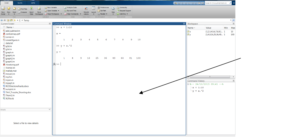
Command
Window

Simple Expressions
To start with try entering the following simple expressions into the command window.
The double arrow on the left (>>) is the MATLAB prompt and will appear after you have
entered each expression. Enter the three expressions pressing return after each of the
expressions.
>> 1 + 2
>> 5^2
>> 7^2 + 5*7 -3
I suspect you have realized that you have just carried out the following calculations.
1+2=3
5
2
=25
7
2
+5×7−3=81
The basic mathematical operators are
Addition +
Subtraction -
Multiplication *
Division /
Raise to a power ^
The order of precedence is that powers are evaluated first, followed by multiplication and
division, with addition and subtraction last. Round brackets can be used to change the
order of precedence.
Calculations within brackets take precedence over everything else.
>> (1 + 2)^2
ans =
9
When there are two items with the same level of precedence, the order is from left to
right.
>> 12/3*4
This means
4
3
12
and not
43
12
because the division operation is to the left of the
multiplication operation.
7
Assignments
An assignment takes the value of an expression and stores it in a variable.
For example :-
>> x = 1 + 2
>> a = 5^2
>> y = 7^2 + 5*7 -3
Once a variable has been created, you can use them in expressions.
>> x^2
>> y = x^2 + 5*x -3
The first character of a variable name must be a letter. Other characters may be numbers
or underscores. The variable name has a maximum length of 63 characters.
If you do not assign an expression to a variable, it is automatically assigned to a variable
called “ans”, which can be used in subsequent expressions.
You may have noticed that each time you enter an expression; the result is printed in the
command window. This is not always desirable. For example, the expression may be in a
program where you don’t want to print intermediate results. Later we will be using arrays
and matrices. Results from these calculations may cover several pages. To suppress the
result being printed out, place a semicolon at the end of an expression. For example :-
>> x = 1 + 2 ;
>> a = 5^2 ;
>> y = 7^2 + 5*7 -3;
Output Display Format
The format command is used to change the way in which numbers are displayed.
format short 5 digit floating point. The default.
format Same as above.
format short e 5 digit scientific notation.
format long 15 digit floating point.
format long Ee 15 digit scientific notation.
8

Mathematical Functions
There are hundreds of functions in MATLAB. To get started consider the standard
mathematical functions that you would expect to find on a calculator.
abs(x)
The absolute value or complex
magnitude.
sqrt(x) The square root.
round(x) The value rounded to the nearest integer.
rem(x,b) The remainder of x divided by b.
sin(x) The sine.
cos(x) The cosine.
tan(x) The tangent.
asin(x) The arcsine. The inverse of sin(x)
acos(x) The arccosine.
atan(x) The arctangent.
exp(x) The exponential base e.
log(x) The natural logarithm. ie to the base e
log10(x) The log base 10.
Trigonometric functions all use radians. However, there are degree based versions of
each of the functions. There name is the same as the functions above, except for and
extra "d" at the end of the name.
>> sind(45)
Functions can be used in any expression in any place you could put a number or a
variable.
>> sin(x)^2 + cos(x)^2
>> 10^(log10(3) + log10(4))
The argument of a function (x and b in the table above) can also be an expression.
>> r = sqrt(3^2+4^2)
The argument can also contain calls to other functions.
>> exp(2*log(3) + 3*log(2))
9

Special Number Symbols
There are symbols in MATLAB that are used to indicate special numbers.
pi
π
inf
∞
NaN Not a number
There are also the symbols used in complex calculations.
i
1
j
1
Mathematicians use i to represent the square root of minus one while in electronics they
prefer to use j. In the next section we will be looking at how to use MATLAB to carry out
complex calculations.
Complex Numbers
Complex numbers can be entered in either Cartesian or polar form.
>> z = 3 + 4i
>> w = 5 * exp(i * pi/6)
or
>> w = 5*(cos(pi/6)+j*sin(pi/6))
Complex arithmetic is carried out with the normal arithmetic operators. MATLAB
automatically detects if a calculation contains complex numbers and carries out the
appropriate calculation.
There are also functions that allow you to obtain particular properties of the complex
number.
real(A) The real part of A
imag(A) The imaginary part of A
conj(A) The complex conjugate of A
abs(x) The modulus of A.
angle(A) The phase angle of A
10
Matrices
The fundamental unit of MATLAB is a matrix. In fact MATLAB is short for matrix
laboratory. However, its use is not restricted to matrix mathematics. Matrices in
MATLAB can also be regarded as arrays of numbers. You can regard matrices as a
convenient way of handling groups of numbers. A matrix in MATLAB can have one, two
or more dimensions or be empty. A matrix with a single element is a special case. They
are treated as a single number. A matrix element can be an integer, a real or a complex
number. You do not have to worry about element types. MATLAB will set the element
type to what is required. Matrices that contain a single row or column are called vectors.
164122302.83
2121321113.17
545411.42253
2.46377657
44925726.4
42.78.8751
i
i
i
i
01.1
5
17
8.8
18
12
Matrix Column Vector
89.31721512
i
34.2
Row Vector Single Number
When specifying the position of an element or the size of a matrix, the convention is to
specify the row before the column. To remember this, I remember R before C like in
“Roman Catholic”.
11
Entering Matrices
To enter the contents of a matrix :
Enclose the contents in square brackets.
Separate each element by white space or a comma.
Separate each row by a semicolon or a new line.
Here are various ways of entering into x a matrix containing
987
654
321
>> x = [ 1, 2, 3; 4, 5, 6; 7, 8, 9]
>> x = [ 1 2 3
4 5 6
7 8 9 ]
>> a = [ 1 2 3 ]
>> b = [ 4 5 6 ]
>> c = [ 7 8 9 ]
>> x = [ a ; b ; c ]
>> x = [ 1, 2 3
b ; c]
You can increase the size of a matrix by adding rows or columns.
For Example :
>> x = [ x ; 10 11 12]
When adding a row to matrix, the number of elements in the additional row must be the
same as the number of elements in each row of the matrix. The same is true for columns.
When you enter a matrix, each of the elements can be entered as an expression.
>> a = [ exp(0) sqrt(4) 1+2 ]
12

Matrix Operations
These operations treat each of the operands as a matrix :-
Matrix Addition +
Matrix Subtraction -
Matrix Multiplication *
Right Matrix Division /
Left Matrix Division \
Raise to a power ^
Transpose matrix ‘
To understand what is going on, let’s look at some examples.
>> A = [ 1 2 ; 3 4];
>> B = [ 5 6 ; 7 8];
This produces two matrices that we can use in the examples.
43
21
A
87
65
B
>> A + 5
This adds 5 to each element of A.
98
76
5453
5251
5
43
21
>> A + B
This adds each element of A to the corresponding element in B.
1210
86
8473
6251
87
65
43
21
>> A - B
This subtracts each element of B from the corresponding element in A.
44
44
8473
6251
87
65
43
21
13
>> A * 5
This multiplies each element in A by 5
2015
105
5453
5251
5
43
21
>> A * B
Multiply matrix A by B.
5043
2219
84637453
82617251
87
65
43
21
>> A ^ 2
Multiply matrix A by itself.
2215
107
44233413
42213211
43
21
43
21
>> A'
Transpose matrix A. Swap rows with columns.
42
31
'
43
21
14

Matrix Division
Matrix division is not something that you find in normal mathematical text book. As you
would expect, matrix division is the inverse of matrix multiplication. What is not so
obvious is that matrix division is the same as solving a set of simultaneous equation. For
example, take the pair of equations:
1143
52
21
21
xx
xx
In matrix form this becomes :
11
5
43
21
2
1
x
x
bAx
Where
43
21
A
2
1
x
x
x
and
11
5
b
If you multiply both sides by
1
A
(the inverse matrix of A).
bAx
bAAxA
\
11
In MATLAB you enter :
>> A = [ 1 2 ; 3 4 ];
>> b = [ 5 ; 11 ];
>> A\b
You need to be careful because matrix multiplication is not commutative. That is to say in
general
BA
does not equal
AB
. That is why there are two division operators.
Left Division Right Division
bAbA
1
\
1
/
bAAb
Divide b by A.
The divide is to the left of b.
Divide b by A.
The divide is to the right of
b.
15

Array Operations
These operations act on corresponding pairs of elements in each of the operands. To
distinguish them from the matrix operations, each is preceded by a dot.
Array Multiplication .*
Right Array Division ./
Left Array Division .\
Raise to a power .^
The operands must be the same size, unless one of the operands is a single number.
You may want to compare the following examples with the examples of matrix operations.
>> A .* B
Multiply each element in A by the corresponding element in B.
3221
125
8473
6251
87
65
*
43
21
>> A ./ B
Divide each element in A by the corresponding element in B.
5.04286.0
3333.02.0
8/47/3
6/25/1
87
65
/
43
21
Array operations are commutative. Therefore A./B = B.\A
>> A .^ 2
Square each element in A
169
41
43
21
2^
43
21
22
22
>> A .^ B
Raise each of the elements in A to the power of the corresponding element in B.
655362187
641
43
21
87
65
^
43
21
87
65
16

Matrices and Functions
If you apply an arithmetic function to a matrix, then the function is applied to each of the
elements in the matrix.
>> sqrt(A)
The square root of each element in A
43
21
43
21
sqrt
>> sin(A)
The sine of each element in A
4sin3sin
2sin1sin
43
21
sin
>> exp(A)
The exponent of each element in A
43
21
43
21
exp
ee
ee
However there are functions that act on the whole matrix. They are only defined for
square matrices.
sqrtm(x) The matrix square root.
expm(x) The matrix exponential base e.
logm(x) The matrix natural logarithm.
17
Help
There are over a thousand different functions in MATLAB and many more in additional
toolboxes. So the ability to find the function you need and learn how to use it is a very
important to MATLAB users. Fortunately there are many ways of finding help, the most
important of which are mentioned below.
Command line help
In the command line you can just enter help and the name of the function.
>> help log
>> help exp
A description of the function and how to use it will be printed in the command window.
The problem with the help command is that you don't always know the name of the
function you are looking for. In that case, you use the lookfor command.
>> lookfor average
If you do this you will find that there is a function call mean that returns the average.
You can then use the help command to find out how to use mean.
>> help mean
There are also hundreds of demo programs on the system that you can use for inspiration.
To see them enter demo in the command window.
>> demo
18

The Help menu
Everything that is in the command line help and much more is available in the MATLAB
documentation. To see the documentation, click on the question mark icon on the home
banner.
Then click on MATLAB.
You can search the documentation by clicking on the Search Documentation text and
entering what it is you want to search for, then click on the blue magnifying glass.
Click on the contents icon a few times to see what it does.
Contents Search
19

Utility Matrices
These functions are used to create standard matrices.
zeros(n) n by n matrix where each element is zero.
zeros(m,n) m by n matrix where each element is zero.
ones(n) n by n matrix where each element is one.
ones(m,n) m by n matrix where each element is one.
rand(n) n by n matrix of random numbers.
rand(m,n) m by n matrix of random numbers.
eye(n) n by n identity matrix.
Generating Vectors
It is often useful to produce a row vector (a matrix containing only one row) containing a
sequence of numbers. A colon can be used to produce a sequence containing two
integers and all the integers in between.
>> x = 1 : 5 generates a row vector x = [ 1 2 3 4 5 ]
A third term in between the other two can be used to specify the gap between each
number.
>> w = 0:0.25:1 generates w = [0 0.25 0.5 0.75 1]
>> y = 0:5:20 generates y = [0 5 10 15 20]
>> z = 6:-1:1 generates z = [6 5 4 3 2 1]
There are also functions that can generate vectors. The function linspace produces a
vector with a specified number of elements.
>> y = linspace(start,end,n)
This produces an evenly spaced vector with n elements. The first element is “start”, the
last is “end”.
>> y = linspace(0,10,5) generates y = [0 2.5 5 7.5 10]
The function logspace produces a vector with a logarithmic distribution.
>> y = logspace(d1,d2,n)
This generates a row vector with n elements logarithmically spaced between
1
10
d
and
2
10
d
.
>> y = logspace(-1,2,4) generates y = [0.1 1 10 100]
20
Subscripts
Subscripts are used to access individual elements of a matrix or produce a sub matrix
from a matrix. They can be used to assign a value to an element or to read the contents
of an element. As an example, consider the matrix A.
1211109
8765
4321
A
An individual element can be read or written to by specifying the row and column in
parentheses after the variable name. To read the element in the second row and third
column of A, you would write :
>> A(2,3)
This would return 7. To change the 7 to 100 you could enter :
>> A(2,3)=100;
1211109
810065
4321
A
Multiple elements can be accessed at a time. A vector can be used to specify a range of
rows or columns.
>> A(2,[1 2 4]) Returns [5 6 8]
1211109
7
4321
865
Vector notation can be used to specify the range.
>> A(1:2,3) Returns
7
3
1211109
865
421
7
3
A colon is used to specify every element of the corresponding row or column.
>> A(3,:) Returns
1211109
1211109
8765
4321
21

If you use subscripting on a vector, then you only need to specify one dimension.
>> B=10:15
151413121110
>> B(2) Returns 11
1514131210
11
>> B([2,4]) Returns
1311
15141210
1311
>> B(4:end) Returns
151413
151413
121110
You can also use the result of a comparison as a subscript. Suppose that we want to find
all numbers in B that are greater than 13. First we compare B with 13.
>> p = B > 13 Returns
110000
Here a one indicates that the comparison is true. In this case, the elements of B that are
greater than 13. A zero indicates that the comparison is false.
Now p can be used as a subscript, to extract all elements where the comparison is true.
>> B(p) Returns
1514
1514
13121110
Relational and Logical Operations
As we have seen above, we can compare a number with each element in a matrix.
You can also compare pairs of corresponding elements in two matrices of equal
dimensions.
The result is a matrix of zeros and ones. They return one for TRUE, or zero for FALSE.
Less than <
Less than or equal <=
Greater than >
Greater than or equal >=
Equal ==
Not equal ~=
Once you have the results of such an operation, you can carry out Boolean logic
operations on them.
AND &
OR |
NOT ~
22

Variable Control Commands
who List all variables in memory.
whos Same as above but with more information.
clear Remove all variables from memory.
clear <variable> Remove specified variables from memory.
For example
>>x = 1; y = 2; z = 3;
>> whos
Name Size Bytes Class Attributes
x 1x1 8 double
y 1x1 8 double
z 1x1 8 double
>> clear x y;
>> whos
Name Size Bytes Class Attributes
z 1x1 8 double
File Control Commands
dir List contents of current directory.
ls List contents of current directory.
what List the Matlab files in the current directory.
cd <directory> Change the current directory.
type <filename> Display the contents of a text or .m file.
delete <filename> Delete a file.
diary <filename> Record all commands and results to a file.
diary off Stop above.
23

Saving, Exporting and Importing Data
MATLAB can load and save data in several different file formats. It has its own binary
data format that can only really be understood by MATLAB. Files of this type have a
".mat" extension. It can also use ascii text files. These are files containing numbers
written in the standard ASCII text, like you would produce in note pad or a text editor.
Columns are separated with white space and each row is on a separate line. MATLAB
will also read and write comma separated value(.csv) files.
save Save all variable to the file matlab.mat
load Load in variables from the file matlab.mat
save <filename> Save all variable to the file filename.mat
load <filename> Load in variables from the file filename.mat
save <filename> <variable>
Save only the variable variable to the file
filename.mat
load <filename> <variable>
Load in only the variable variable from the
file filename.mat
save <filename> <variable> -ascii Save variable to the text file filename
load <filename>.<ext>
Load from the text file, to a variable called
filename
save <filename> <variable> -ascii
-double
Save variable to the text file filename using
double precision.
csvwrite(<filename>.cvs , M) Write matrix M to csv file.
M=csvread( <filename>.csv) Load from the csv file, into variable M
Matlab can also read in other file formats. For more information, enter
doc 'Supported File Formats'
in the command window.
24

The Desktop
Almost anything you want to do in MATLAB can be done from the Command Window.
However, there are numerous other windows that can make certain procedures simpler. If
you look at the MATLAB window on a computer, it will look something like this.
You can drag windows around, remove them and resize them. The MATLAB layout is like
a Rubik's cube, three moves and it is very difficult to get back to where you started.
However, you can always select Layout ►Default on the banner, under the Home tab.
Command History
This shows all the previous commands that you have entered in the command window.
Double clicking on a command in this window will execute the command. You can also
drag the command back into the command window, edit them and run them again.
Another way of doing this is to use the up and down cursor keys in the command window
to recall previous commands. You can then use the left and right cursor keys and the
delete key to edit the command.
You can also use the Command History to create a program file. Hold down the ctrl key
and click on each of the commands that you want in the file. Then right click and select
Create Script. The selected commands will be copied into the MATLAB editor.
25
Info on highlighted file
Command History
Workspace
Current FolderFiles in Current
Folder

Workspace
The Workspace window is a variable explorer. Clicking on a variable with the right mouse
button allows you to rename or delete a variable. If you double click on a variable, it
opens a Variables Editor that allows you to change the contents of a variable.
Current Folder
Like most operating systems, MATLAB uses the concepts of a path and a current
directory (folder). The path is a list of directories where MATLAB will search for files. The
path is set when you install MATLAB to include all the necessary directories in the
MATLAB installation. MATLAB also includes the current folder in the search path. While
it is possible to add directories to the path (See Search Path in MATLAB help) the most
common way of ensuring that MATLAB can see your files is to change the current folder
to the required location.
To change the current directory(folder), you can use the cd command, like you would in
windows, Linux or OSX. However, I find the box at the top of the MATLAB window more
convenient to use.
Associated with this is the Current Folder
Window. This window is like a file manager or
windows explorer.
• Double clicking on a .m file will open the
file in the MATLAB editor.
• Double clicking on a .mat file will load
the variables stored in the file.
• Double clicking on a folder will set the
current directory to that folder.
• Double clicking on a Excel file will open
the file import window.
You can create new files and folders by right
clicking on the window background.
If you right click on a file or folder, you can
select to rename or delete the file or folder.
You can also use this method to run a MATLAB
program or import data from a file.
26
Browse
Up one level
Select Drive
Select Folder
Recall previous settings

MATLAB as a Programming Language
So far we have treated MATLAB like a super calculator. However, every command and
expression we have used so far can be used in a MATLAB program. In this sense the
commands and expressions of MATLAB can be regarded as a programming language.
MATLAB has all the constructs you would expect in a programming language, such as
loops, functions and conditional execution. These programs are stored in files with a ".m"
suffix. For this reason they are general called M files. There are two types of M files,
scripts and functions.
Script M Files
A MATLAB script is a file containing a list of MATLAB commands. The commands in the
script are executed by entering the name of the file without the ".m" suffix. The easiest
way to create an M file is to use the editor. Try the following. At the matlab prompt enter
>> edit myscript.m
In the editor, enter
x = linspace(0,2*pi,100);
y = sin(x);
plot(x,y);
Then save. At the matlab prompt enter the name of the script to run it.
>> myscript
You can add your own comments to the script. Place a percent sign (%) before each
comment. Everything after the percent sign on that line is regarded as a comment.
Comments are displayed in green in the editor.
You may find these functions and commands useful within a script.
A = input( 'What is A ?
');
Ask the user for a number.
pause Wait for the user to press a key.
pause(5) Wait for 5 seconds
! command Execute and operating system command
display(a) Suppose a = 5. This would print "a = 5";
disp(a) Same as above, but with out the "a = ".
27
Function M Files
If an M file has the word "function" on the first line, then the file contains a definition of a
MATLAB function. Here is a listing of a file called corner.m.
function y = corner(x)
% CORNER the corners of a matrix.
% corner(x) returns a two by two matrix containing the values
% in each of the four corners of x.
[n,m]=size(x); % The number of rows and columns of x
y = [ x(1,1) x(1,m) ; x(n,1) x(n,m) ];
The first line specifies that the function name is "corner" and that "x" is an input parameter
and "y" is the return value. The next three lines are comments. These lines are used by
the help command, they will be printed out if you type "help corner". The rest of the file
contains the commands to implement the function. The last line assigns a value to "y"
which is returned. The variable "n" and "m" are local to the function. They cannot be
accessed outside the function. This function can now be used in an expression in the
same way as any other function.
>> corner(p)
>> c = corner(w);
>> help corner
You may have noticed that we used a function called size. This returned the number of
rows and the number of columns of the matrix x. Unlike some programming languages,
MATLAB functions can return more that one item. The following example shows how you
would write a function that returns many items.
function [sum,difference] = add_subtract(a,b)
sum = a + b;
difference = a - b;
To call this function, you would enter :-
>> [s d] = add_subtract(1,2)
The variable "s" contains the sum, and "d" the difference.
28
Flow Control
So far, all the programs have consisted of lines of statements carried out in sequential
order. However, most programs will need to be able to select conditionally which
instructions to execute and repeat part of the program several times by using a loop.
MATLAB has enumerated loops (for loops), precondition loops (while loops) and
conditional execution (if statements).
Enumerated Loops (for)
Enumerated loops are used to repeat a sequence of statements a known number of times.
for x = 1:10
y(x) = x.^2+3*x+5;
end
The middle line is the statement to be repeated. Here it is only one line, but it could just
as easily be several lines. Any line between for and end is repeated. The loop is
repeated for each item in an enumerated sequence. In this case the sequence is the
numbers one to ten. Each time around the loop, the loop counter variable "x" is assigned
one of the numbers in the sequence, in order. So the first time around the loop, "x" will be
one, the next time around the loop it will be two, then three, then four, up to ten.
In most programming languages, the enumerated sequence is defined by stating a rule for
finding the next number in the sequence. The enumerated sequence in MATLAB is
defined by a vector. Which means you can use a sequence with no logical connection
between items in the sequence.
A = rand(1,5);
for a = A
disp(a)
end
for k = [ 1 7 3 pi i]
disp(k)
end
The general form of a for loop is :-
for <variable> = < vector>
<statement>
<statement>
etc
end
New MATLAB users, especially those that have experience of computer programming,
tend to over use for loops. The first example can be achieved much more efficiently
without using a loop at all.
>> x = 1:10
>> y = x.^2+3*x+5;
29

Precondition Loops (while)
A precondition loop is used to repeat a sequence of statements zero, one or more times.
Unlike the enumerated loop, the number of repetitions is not a fixed quantity and can
change as the loop runs.
The following example shows how to use a precondition loop to implement an iterative
process.
A = 7; %Want to find the square root of A.
x=1; %First guess
err=1; %Set error to something to get started
while(err>0.0001)
x = (x.^2+A)./(2*x); %Iteration equation (Newton Raphson)
err = abs(A-x.^2); % calculate the error
end
disp(x);
The loop consists of all the statements in the lines between while and end. The condition
in the brackets to the right of while determines if the loop is going to execute or not. First
the condition is evaluated. If the result is true (non zero) then the two lines below the
while are executed. The program then goes back to the start of the while loop and
evaluates the condition again. The loop will keep repeating until the result of the condition
evaluates to false (zero). When this happens the lines between while and end are not
executed. The program jumps to the first line after the end.
Below is the general form of a while loop.
while(<condition>)
<statement>
<statement>
etc
end
You loop while the condition is true.
You can put in as many statements as you like in the
loop. The loop can include other while loops, for loops
and if statements.
condition
statement
statement
True
False
30
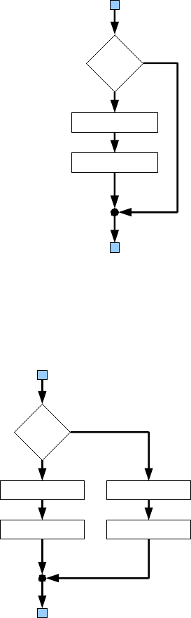
Conditional Execution (if)
The if statement is very like a while loop, except that it will only run
once if at all.
if(<condition>)
<statement>
<statement>
etc
end
If the condition is true, the statements inside are executed. They
will notbe executed if the condition is false. In either case, the if
statement is then finished and the program goes to the next line in
the program. The following example finds the absolute value of the
variable A.
if (A<0) % If A is negative
A = -A; % Make A Positive
end
There is another form of if statement
if(<condition>)
<statement>
<statement>
etc
else
<statement>
<statement>
etc
end
If the condition is false, the statements after the else are
executed.
For example
if (A<B) % If A is negative
disp('A is less than B')
else
disp('A is not less than B')
end
You can put in as many statements in the conditional parts as you like.
These can include while loops, for loops and other if statements.
condition
statement
statement
True
False
condition
statement
statement
True
False
statement
statement
31

Graph Commands
This section describes how you can produce graphs in MATLAB. The script below shows
how to plot and annotate a simple graph.
% Matlab Script to plot a Sin Wave
% Create the x and y vectors to plot
x = 0:6:360 ; % The values of x in degrees
rads = 2*pi*x./360; % The above convert to radians
y = sin(rads); % Calculate the values of y
plot(x,y); % Plot the graph
% Annotate the graph
title('Sine Wave'); % Add a Title
xlabel('degrees'); % Label the x axis
ylabel('value'); % Label the y axis
grid; % Draw a grid on the graph
axis([0 360 -1 1]); % Set the limits of the x and y axis
Running this script produces the following graph
32

2D Graphics Commands
The plot command produces a linear x-y plot. Listed below is a selection of plot
commands.
plot(y) Plot y against the element number.
plot(x,y) Plot y against x.
plot(x1,y1,x2,y2) Plot y1 against x1 and y2 against x2.
You can use a third argument to define various options.
plot(x,y,'r+') Plot y against x using red plus signs.
plot(x1,y1,'r+',x2,y2,'go') Use red plus signs for x1 and y1
and green circles for x2 y2.
Plot options are used to define the line type or point type and the colour. Plot options are
enclosed in quotes to distinguish them from variables.
Symbol Point or Line
Type
Symbol Colour
. Points y Yellow
o Circles m Magenta
x X marks c Cyan
+ Plus Signs r Red
* Stars g Green
- Solid Line
(Default)
b Blue
(Default)
: Dotted Line w White
-. Dash dot Line k Black
-- Dashed Line
The plot options can be one, two or three characters long. For example 'rx-' will plot x
marks and a solid line, both in red.
In addition to the plot command, there are other commands to produces other types of 2 D
graphs. On the next page are various examples of the graphs produced by the
commands fill, bar, stairs, etc.
The arguments and options of these commands are similar to those of plot.
33

34
Subplots
Subplot enables you to split the graphics window into a number of smaller subgraphs.
As an example, consider how the graphs where plotted on the previous page.
subplot(4,3,1); % 4 by 3 graphs, 1st graph
fill(degrees,sin(rad),'g'); % Plot a Fill graph
The subplot command has three arguments. The first digit specifies the number of rows
of graphs you want and the second the number of columns. In this case we are going to
have 4 rows of graphs in 3 columns. The third number specifies which of the 12
subgraphs you are going to use next. The subgraphs are numbered from left to right, top
to bottom. So the Fill plot will be in the top left had corner. Next to it is the bar plot.
subplot(4,3,2); % 4 by 3 graphs, 2nd graph
bar(degrees,sin(rad),'g'); % Plot a Bar Graph
and so on.
subplot(4,3,3); % 4 by 3 graphs, 3rd graph
stairs(degrees,sin(rad)); % Plot a Stair Graph
subplot(4,3,4); % 4 by 3 graphs, 4th graph
etc
Figure
An alternative to splitting a window into several graphs is to open a new window.
MATLAB calls a graphics window a figure. To open a new figure, you use the figure
command.
figure; % Open a new window.
This opens a new figure, which becomes the current graphic window. Any subsequent
plots will be drawn in the new figure. Figures are numbered 1,2,3 etc, which is called the
handle. The figure command returns the handle of the new figure.
h=figure; %h is the handle of the new figure.
The figure command can also be used to set the current figure to an existing figure.
figure(h); %Set the current figure to h.
Here are some other commands that are useful for managing figures.
clf Clear the current figure.
clf(h) Clear figure h.
h = gcf Get the handle of the current figure
delete(h) Delete figure h.
35
Hold
The hold command enables you plot a graph over the top of another graph. In the default
state, when a new graph is plotted, the old graph is removed first. The hold command
stops the removal of the old graph. Any subsequent graphs are plotted on top of each
other using the same axis.
hold on Hold the plot on the screen.
hold off Release the plot on the screen.
hold Toggle the hold state.
Conclusion
This seminar by necessity is fairly restricted. It has only covered a very small fraction of
MATLAB commands and functions. If you want to get some idea of what else is in
MATLAB, scroll through the function reference in Help. We have not even touched on
any of the toolboxes. However, don't let that put you off. Very few people, if any body
knows how to use all the functions within MATLAB. The seminar includes the
fundamental basic commands and operations that you need to use the software. These
should be sufficient to cover most, if not all of your requirements.
Although this seminar can only deal with the basics, it has a secondary aim of showing
you ways of finding out more information. If you want to use some of the more specialized
areas of MATLAB like Statistics, 3D graphics, graphical user interfaces, etc, I hope that
you now have a better idea where you go to find out how to do it. On the next page you
will find various links that can provide you with additional information.
You should now be able to use MATLAB interactively and to write your own functions and
scripts, perhaps using this document as a reference. Like most skills, it is practise that is
required. So I hope that you will go back to your own computer and start using it.
36

Further Information
If you want to know more about using MATLAB, always try looking in help first. In
particular, there are links to video tutorials. You will find these at
http://uk.mathworks.com/help/index.html
The Oxford University MATLAB Portal
This is a one stop shop for MATLAB users in the University of Oxford.
https://uk.mathworks.com/academia/tah-portal/university-of-oxford-30972477.html
MATLAB Academy Online Training Suite
This includes over 60 hours of online training courses for different levels and across
different subject categories. See the MATLAB portal above.
MATLAB course at University of Oxford, IT Services
IT Services run a course called Matlab: A comprehensive introduction
https://help.it.ox.ac.uk/courses/overview
University Licences
For an overview of the various ways to license MATLAB within the University, see:
http://www.eng.ox.ac.uk/~labejp/TAH/matlabTAH.html
37
