
MICROSIMULATION TOOLS FOR THE
EVALUATION OF FISCAL POLICY
REFORMS AT THE BANCO DE ESPAÑA
Documentos Ocasionales
N.º 1707
Olympia Bover, José María Casado,
Esteban García-Miralles, José María Labeaga
and Roberto Ramos
2017
MICROSIMULATION TOOLS FOR THE EVALUATION OF FISCAL POLICY REFORMS
AT THE BANCO DE ESPAÑA
MICROSIMULATION TOOLS FOR THE EVALUATION OF FISCAL
POLICY REFORMS AT THE BANCO DE ESPAÑA
Olympia Bover, José María Casado, Esteban García-Miralles
and Roberto Ramos
BANCO DE ESPAÑA
José María Labeaga
UNED
Documento Ocasional. N.º 1707
2017
The Occasional Paper Series seeks to disseminate work conducted at the Banco de España, in the
performance of its functions, that may be of general interest.
The opinions and analyses in the Occasional Paper Series are the responsibility of the authors and,
therefore, do not necessarily coincide with those of the Banco de España or the Eurosystem.
The Banco de España disseminates its main reports and most of its publications via the Internet at the
following website: http://www.bde.es.
Reproduction for educational and non-commercial purposes is permitted provided that the source is
acknowledged.
© BANCO DE ESPAÑA, Madrid, 2017
ISSN: 1696-2230 (on line)
A
bstract
This paper presents the microsimulation models developed at the Banco de España for the
study of fiscal reforms, describing the tool used to evaluate changes in the Spanish personal
income tax and also the one for the value added tax and excise duties. In both cases
the structure, data and output of the model are detailed and its capabilities are illustrated
using simple examples of hypothetical tax reforms, presented only to illustrate the use of
these simulation tools.
Keywords: microsimulation, Spain, personal income tax, value added tax, excise duties.
JEL Classification: C81, D12, H20.
Resumen
Este documento presenta los modelos de microsimulación desarrollados por el Banco de
España para el estudio de reformas fiscales. Por un lado, describe la herramienta
de microsimulación que evalúa cambios en el impuesto sobre la renta de las personas físicas
(IRPF). Por otro lado, explica la herramienta del impuesto sobre el valor añadido (IVA) y los
impuestos especiales. Para cada una de estas dos herramientas, el documento detalla cómo se
estructura, los datos usados y los resultados que genera. También se muestran las capacidades
de estas herramientas mediante ejemplos sencillos de reformas fiscales hipotéticas, presentadas
exclusivamente para ilustrar el uso de estos simuladores.
Palabras clave: microsimulación, España, IRPF, IVA, impuestos especiales.
Códigos JEL: C81, D12, H20.
INDEX
Abstract 5
Resumen 6
1 Introduction 8
2 The Banco de España Personal Income Tax Microsimulation Model 10
2.1 The data 10
2.2 Framework of the Banco de España Personal Income Tax Microsimulation Model 11
2.2.1 The Spanish personal income tax 11
2.2.2 Parameters 14
2.2.3 Adjustment of the data in order to construct the 2015 baseline scenario 15
2.2.4 The output of the model 15
2.2.5 The accuracy of the model 15
2.2.6 Baseline results: personal income tax revenues and the distribution of tax
liabilities under the 2015 legislation 16
2.3 Simulation example 17
3 The Banco de España Indirect Tax Microsimulation Model 22
3.1 The data 22
3.2 Framework of the Banco de España Indirect Taxation Microsimulation Model 23
3.2.1 The value added tax and excise duties 23
3.2.2 Parameters 23
3.2.3 The demand system: behaviour in the Banco de España Indirect taxation
microsimulation model 28
3.2.4 The output of the model 32
3.2.5 The accuracy of the model 32
3.2.6 Baseline Results: indirect tax revenues and the distribution of tax liabilities
under the 2015 legislation 32
3.3 Simulation examples 35
3.3.1 A Change in VAT: a one point increase in the standard VAT rate 35
3.3.2 A Change in excise duties: an increase in the ad quantum tax on spirits 38
4 Conclusions 41
References 42
BANCO DE ESPAÑA 8 DOCUMENTO OCASIONAL N.º 1707
1 Introduction
This paper presents the microsimulation models developed at the Banco de España (BdE) for
the study of fiscal reforms involving changes in personal income taxation (PIT) and indirect
taxation (VAT and excise duties). The aim of the paper is to present the main features of the
tools and illustrate their capabilities using simple examples of tax reforms.
Microsimulation models are tools that simulate the effect of a reform on a representative
sample of individual agents (taxpayers, households, firms, etc.). They allow the aggregate and
the distributional effects of tax reforms to be studied, taking into account the heterogeneity
among individuals. As a consequence, they are a powerful tool for the development of decision-
support models in order to simulate and evaluate the impact of public policies.
Spurred by the availability of micro data and computer power, the use of
microsimulation methods to perform ex-ante and ex-post evaluation of fiscal reforms is
becoming more and more widespread. Currently, there is an extensive array of policy and
research institutions in Europe that have developed and maintain such models, such as the
Institute for Fiscal Studies in the UK (TAXBEN), the Institut des Politiques Publiques in France
(TAXIPP), the CPB Netherlands Bureau for Economic Policy Analysis (MIMOSI) and the Institute
for Social and Economic Research at the University of Essex, in collaboration with national
teams (EUROMOD, the European Commission sponsored tax-benefit microsimulation model),
to name a few. Microsimulation techniques can contribute to current fiscal policy debates and,
especially when it comes to modelling behavioural responses triggered by tax reforms, they
have attracted a lot of attention from the academic community.
The microsimulation model of direct taxation developed at the Banco de España
allows morning-after (first-round) aggregate and distributional effects of reforms in the Spanish
personal income tax (Impuesto sobre la Renta de las Personas Físicas or IRPF) to be
simulated. It allows a wide range of reforms stemming from changes in the parameters of the
tax code to be evaluated, in the absence of any behavioural reaction by agents.
In Spain, the first arithmetic microsimulation model of direct taxation was MOSIR
(Modelo de Simulación del Impuesto sobre la Renta) developed by Castañer and Santos (1992)
at the Instituto de Estudios Fiscales (IEF) using administrative records. Levy et al. (2001)
presented ESPASIM, a microsimulation model of direct taxation, as well as of social
contributions, indirect taxation and excise duties. The database for the microsimulator of direct
taxation was the ECHP. In the early 2000s the IEF created a microsimulation unit that built
SIRPIEF, which performed both arithmetic and behavioural simulations based on survey data
from the ECHP. A summary of this tool is contained in Sanz et al. (2004) and their labour
supply model borrows from Labeaga and Sanz (2001). Oliver and Spadaro (2004) developed
GLADHISPANIA, a combined arithmetic-behavioural tool based on data from the ECHP. Also
at the IEF, Moreno et al. (2010) developed Microsim-IEF, and Onrubia et al. (2013) developed
MODELAIR, both arithmetic models using administrative records. There are many other
applications of microsimulation that use Spanish direct-taxation data as well as tax-benefit
models. Some examples are presented by García et al. (1997), Badenes et al. (1998) and
García and Suárez (2002, 2003).

BANCO DE ESPAÑA 9 DOCUMENTO OCASIONAL N.º 1707
The Banco de España microsimulation model for indirect taxation allows changes in
the value added tax (Impuesto sobre el Valor Añadido or IVA) and excise duties (impuestos
especiales) to be simulated. In addition to morning-after effects, it captures the behavioural
response of households through the estimation of a demand system. Therefore, in addition to
first-round effects, the tool allows households’ behavioural reaction to price changes stemming
from a tax reform (second-round effects) to be predicted.
In Spain, the first tool for indirect taxation was developed by Labeaga and López
(1995), whose complete demand model was presented in Labeaga and López (1994). The
microsimulation unit at the IEF also developed a tool for indirect taxation, SINDIEF (Simulador
de Impuestos Indirectos del Instituto de Estudios Fiscales). Sanz et al. (2003) provide a
summary of its functioning. Examples of microsimulation papers dealing with indirect taxes and
excise duties are Labeaga and López (1997) and Labandeira and Labeaga (1999). An overall
discussion of microsimulation can be found in Bourguignon and Spadaro (2006), while a
summary for Spain is contained in Ayala et al. (2004).
The models for PIT and for VAT and excise duties both provide a comprehensive
evaluation of tax reforms, by accounting for the effects relating to tax collection, effective
tax rates, winners and losers and inequality indices. These effects are disaggregated by
income decile and age group. Moreover, the model for indirect taxation provides results
for welfare changes.
The rest of this paper presents the two microsimulation models, starting with the
personal income tax model and afterwards the VAT and excise duties model.
1
1 Both tools are accompanied by a User Guide that explains how to execute them in order to simulate different policies.

BANCO DE ESPAÑA 10 DOCUMENTO OCASIONAL N.º 1707
2 The Banco de España Personal Income Tax Microsimulation Model
This model simulates the tax liabilities stemming from the Spanish personal income tax
(Impuesto sobre la Renta de las Personas Físicas or IRPF) for a large representative sample of
taxpayers. The model incorporates most of the tax code specificities that determine the
calculation of tax liabilities. Therefore, it allows a wide range of reforms, such as those involving
marginal tax rates, tax deductions, tax credits, and exemptions, to be simulated.
The model is an arithmetic tool that provides morning-after effects of the reform being
simulated insofar as behavioural effects, such as the variation in employment status or hours
worked, are not taken into account. The outcome of the model includes an estimation of total
tax revenues, winners and losers, and changes in average tax rates by income decile and age
group. Furthermore, it provides measures of inequality and redistribution. It also allows the
simulated micro data to be saved for the performance of further analysis.
2.1 The data
The data used by the model is a (stratified) random sample of 2013 tax returns namely, the
MUESTRA IRPF 2013 IEF-AEAT (Declarantes). As more recent data become available they will
be incorporated into the model updates. The sample size (in 2013) is about 2.2 million tax
returns, which corresponds roughly to 11% of the population. They pertain to the 15 regions
with a common tax regime and the two autonomous cities of Ceuta and Melilla. Therefore, they
exclude the two regions with special tax regimes (the Basque Country and Navarre). For a
detailed description of this dataset see López et al. (2016).
The dataset contains most of the fiscal variables and socio-demographic characteristics
included in the tax return (modelo 100). Therefore, it contains very precise information on income
sources and tax benefits, as well as some family characteristics, such as the number of
dependent children, other dependent relatives, disability and location. The detailed information in
the dataset allows individual tax liabilities to be accurately simulated and a wide range of reforms
to be modelled. Yet the fact that no information on the employment status of the taxpayer is
provided prevents the modelling of behavioural responses following tax reforms.
Tax returns are of two types: single tax returns, filed at the individual level, and joint tax
returns, filed by (mainly) married couples. In joint tax returns, incomes are pooled together and
are eligible for an additional deduction on top of those available for single tax returns. Apart
from these and other small differences, the computation of tax liabilities is similar. The decision
on which type to choose is taken by the taxpayer. In general, joint tax returns benefit couples
when one spouse earns little or no income, as well as single-parent families when the children
do not have any income.
2
The model abstracts from the choice between single or joint tax
returns, taking it as given. In 2013, around 79% of tax returns were single tax returns, the rest
being joint ones.
Table 1 reproduces some of the items included in Table 2 of López et al. (2016). It
shows that the sample aggregates constructed from the micro data provide an accurate
representation of the population aggregates, the differences being smaller than 1.5% in all
cases, except that of save income stemming from gains and losses.
2 Single parents can file a joint tax return despite being only one individual, benefiting from the corresponding deduction.

BANCO DE ESPAÑA 11 DOCUMENTO OCASIONAL N.º 1707
The sample of tax returns is complemented by an additional dataset containing
information on taxes withheld at source corresponding to people with no obligation to file a tax
return and who do not do so, even though they would very likely obtain a refund. This dataset,
known as “no obligados, no declarantes”, is not included in the microsimulation model and
therefore this population is excluded from the simulations. In 2013 it amounted to 2.3 million
persons and €2.1 billion of withholdings.
2.2 Framework of the Banco de España Personal Income Tax Microsimulation Model
2.2.1 THE SPANISH PERSONAL INCOME TAX
The model follows the personal income tax code in order to simulate the tax liabilities of each
taxpayer. Many specific parameters of the tax code are left free in order to allow reforms to be
simulated. When these parameters take the actual value of the tax code, the model replicates
(approximately)
3
the actual tax liability data.
Figure 1 provides a simplified diagram of the tax code in 2013. Gross income subject to
the tax can be of several types: labour income, capital income (both financial and real-estate) and
self-employment income. Certain deductible expenses can be subtracted from gross income,
including, for example, the social security contributions paid by the employee, a given amount for
labour income earners, and economic expenses associated with the business activity.
Gross income net of deductible expenses is classified into two groups, which are
subsequently taxed at different rates. On the one hand, “general income” comprises mainly
labour income, self-employment income and some capital income. On the other hand, “savings
income” includes the largest portion of capital income. To each type of income a set of
deductions is applied. For example, to general income a deduction for joint filing as well as one
for contributions to private pension plans, among others, can be applied. If the taxpayer is
entitled to deduct an amount exceeding her general income, she can apply the remainder
3 Some small deviations between the actual data and the simulation may occur due to rare instances in which
deductions exceed the maximum amount entitled by law or there exist slight discrepancies between the reported data
and the result of the application of the tax code. Also, some tax benefits depend on variables that are either not
observed or are only partially observed, hence some assumptions were made in order to ease the simulation. For
example, siblings filing individual tax returns may be entitled to share the family allowance for parents living with the
taxpayer, depending on the number of months of cohabitation, a variable that is not observed. Hence, a value of
12 months of cohabitation was assumed. Moreover, since some tax benefits depend also on previous variables of the
tax code, errors may accumulate or cancel each other.
ACCURACY OF THE PERSONAL INCOME TAX MICRO DATA TABLE 1
€bn Tax form box
Sample
aggregate
Population
aggregate Difference
Gross monetary labour income 1 375.7 375.5 0.0%
Gross capital income 28+38 18.4 18.4 0.0%
Self-employment income 125+150+180 22.5 22.4 0.4%
Income from gains and losses 361+368 8.0 8.4 -4.8%
General taxable income 415 327.1 327.0 0.0%
Savings taxable income 419 24.7 25.0 -1.4%
Family allowance
(general and savings income) 439+440 109.7 109.8 -0.2%
Tax liabilities
(gross of working mother tax credit) 511 67.0 67.1 -0.2%
SOURCE: López et al. (2016).
BANCO DE ESPAÑA 12 DOCUMENTO OCASIONAL N.º 1707
of some deductions to her savings income. Income minus deductions is the general taxable
income and the savings taxable income.
Two different tax schedules are applied to each type of income, a state schedule and
a regional schedule. This stems from the fact that around 50% of the personal income tax
revenue is transferred to the regions, which are entitled to modify their own tax schedule and to
introduce their own tax credits. In 2013, the general state schedule consisted of 7 tax bands
and a top marginal rate of 30.5%. On top of this, as mentioned, the regional general tax
schedule is applied. For example, that of the Madrid region comprised four tax bands and a
top marginal rate of 21.4%; that of Catalonia had 6 tax bands and a top marginal tax rate of
25.5%. Madrid taxpayers therefore faced a top marginal rate of 51.9%, while taxpayers in
Catalonia were subject to a top marginal tax rate of 56%.
The savings tax schedule is much less progressive. In 2013 the state part consisted of
3 bands and a top marginal rate of 16.5%, whereas the regional part consisted of 2 bands and
a top rate of 10.5%. In this case, the savings regional tax schedule did not vary across regions.
Once the general income tax liabilities are computed (state and regional components),
they are reduced by the family allowance (again, with state and regional variability, although in
this case they are all similar). The family allowance is computed by applying the general tax
schedule to an amount that depends on the characteristics of the taxpayer and her family,
such as her age, number of dependent children, number of dependent parents, and disability
of the taxpayer and of the dependent members of her family.
After subtracting the family allowance, the state general income and state savings
income tax liabilities are pooled together. Similarly, the regional general income and regional
savings income tax liabilities are added together.
To these two types of tax liabilities a set of tax credits is applied, some of which are
state or region specific and some of which pertain to both. Among them are the tax credit on
house purchases (if they were made before 2013), the large set of regional tax credits and a tax
credit for low labour income earners. The state and regional tax liabilities net of these and the
other tax credits are then pooled together.
Finally, to these pooled tax liabilities, which cannot be below zero, a refundable tax
credit is applied in the case of employed mothers with children below the age of three. The final
tax liabilities are obtained after the subtraction of this tax credit.
It must be noted that when running the microsimulation model, the baseline scenario
(against which the reform scenario is compared) is in general the 2015 tax code. As we explain
later, this forces some adjustments to be made to the data. Specifically, we update the sample
weights and the income data by using information on the number of taxpayers by region and
on aggregate income growth by income source, respectively. Moreover, we apply the 2015 tax
code to the adjusted data. This is very relevant, because in 2015 a tax reform was
implemented, involving important changes in the tax code. For example, the number of state
tax bands was reduced from 7 to 5, and the state tax rates were significantly reduced. For
instance, the top state marginal tax rate was reduced from 30.5% to 22.5%. Moreover, some
regions changed their tax schedules. Also, the family allowance was increased and new
refundable tax credits associated with family characteristics were granted. Regarding
deductions, some of them were reduced, for example, the one for labour income earners

BANCO DE ESPAÑA 13 DOCUMENTO OCASIONAL N.º 1707
and that for contributions to private pension plans. All these changes are modelled, whenever
possible, in the microsimulation tool.
SIMPLIFIED DIAGRAM OF THE PERSONAL INCOME TAX CODE (2013) FIGURE 1
BANCO DE ESPAÑA 14 DOCUMENTO OCASIONAL N.º 1707
2.2.2 PARAMETERS
The microsimulation model considers a large set of parameters that characterise the tax code
and therefore determine the computation of tax liabilities. The number of parameters
incorporated in the microsimulation tool is around 1,500, including many specific to each
region. Currently, the personal income tax codes of 2013, 2014 and 2015 are modelled. The
simulation exercise consists in modifying this set of parameters in order to obtain the resulting
tax liabilities under alternative tax codes. Some examples of possible reforms that the model
can simulate are the following.
a) Switching tax benefits off and on
Almost every tax deduction and tax credit is associated with a binary parameter that
determines whether it is applied or not. Therefore, the model can simulate, for
example, a restriction on certain tax benefits. Furthermore, the model can simulate
the conversion of some tax deductions (subtracted from the tax base) to tax credits
(subtracted from the tax liabilities). Also, it allows the form of application of some tax
benefits to be changed, for instance from being a fraction of a particular variable
to being a fixed amount.
b) Changing the upper and lower bounds of tax benefits
The amounts of many tax benefits are restricted by fixed quantities or by a fraction of
other variable(s). As long as the microsimulation includes these restrictions, it allows
them to be modified. It must be stressed that the micro data already incorporate the
actual restrictions, so that the model cannot simulate increases in many tax benefits.
This is the case when the underlying variable giving rise to the benefit is unobserved.
For example, the deduction on the amount of charity donations is capped at €500.
Insofar as the total amount donated is unobserved, an increase in this tax benefit to,
say, €600 cannot be simulated, since it is not possible to know for which taxpayers
the actual restriction is relevant. In these cases, only a reduction (or complete
elimination) of the tax benefit can be simulated.
c) Adjusting the monetary values of tax benefits
For those tax benefits that consist of a fixed monetary value or that depend on
observable characteristics of the taxpayer, the model allows the value of the tax
benefit to be freely adjusted. This is the case, for example, of the large set of family
allowances.
d) Changing the classification of income sources
The model allows changes in the classification of some income sources between
general income and savings income, or their exclusion from taxable income. This is
useful in order to simulate reforms to the manner in which each type of income
is taxed. For example, a change in the way in which capital (savings) income is taxed
to make it the same as for labour income could be simulated.
e) Modifying the tax schedules
The model readily permits modification of the state and regional tax schedules, both
for general income and savings income.

BANCO DE ESPAÑA 15 DOCUMENTO OCASIONAL N.º 1707
2.2.3 ADJUSTMENT OF THE DATA IN ORDER TO CONSTRUCT THE 2015 BASELINE SCENARIO
In the current version of the microsimulation model, the baseline scenario, against which the
reform scenario is compared, usually corresponds to 2015. Given that the data pertain to
the year 2013, this requires an update of the data. In this regard, two adjustments are carried
out. First, the sample weights are adjusted by considering the changes in the number of
taxpayers by region. Second, the income data are adjusted using aggregate income changes
by income source. The source of these aggregate changes is the AEAT.
4
Then, in order to
construct the 2015 baseline scenario, the microsimulation model with the parameters
characterising the 2015 tax code is run on the adjusted micro data. Note also that a similar
procedure is carried out if the baseline scenario chosen is the 2014 tax code. If the baseline is
2013, no adjustment to the data is performed.
2.2.4 THE OUTPUT OF THE MODEL
The model simulates the set of variables comprising the tax return of each sampled taxpayer in
both the baseline and the reform scenarios. It then aggregates certain variables either
by income decile or age group in order to perform some comparisons. Specifically, it provides
information on total revenue, average tax rates, winners and losers, and several inequality
measures, such as the distribution of after-tax income, Lorenz curve, Gini coefficient and some
percentile ratios. A standard output from the model can be observed in the example presented
in Section 2.3. The program also allows the simulated micro dataset to be saved, so that
further analysis can be performed.
2.2.5 THE ACCURACY OF THE MODEL
In this section we compare some aggregates produced by the microsimulation model for
the tax legislation of 2013, 2014 and 2015 with the corresponding aggregates reported by the
Spanish Tax Agency (AEAT). Note that for 2014 and 2015 the data have been updated as
described above. The results are reported in Table 2.
5
As can be seen, for each single item the sample aggregate is very close to the
population aggregate, the largest deviation being only 0.8%. This suggests that the model
yields an accurate description of overall income and tax liabilities.
4 Estadísticas de los declarantes del Impuesto sobre la Renta de las Personas Físicas (IRPF).
5 Table 2 does not include the withholdings from persons under no obligation to file a tax return and who decide not to
do so.
SAMPLE AGGREGATES FROM THE MICROSIMULATION MODEL COMPARED WITH
POPULATION AGGREGATES
TABLE 2
€bn
Model AEAT Difference (%)
2013 2014 2015 2013 2014 2015 2013 2014 2015
Number of tax-payers (million)
19.2 19.3 19.5 19.2 19.4 19.5 -0.1 -0.1 -0.1
Income ("Rendimientos")
421.4 428.2 447.0 421.8 428.6 447.0 -0.1 -0.1 0.0
Tax Base ("Base Liquidable")
351.8 358.0 375.7 352.2 357.2 375.3 -0.1 0.2 0.1
Tax Liabilities before Tax Credits ("Cuota Íntegra")
72.0 73.5 71.0 72.1 73.2 71.0 -0.1 0.4 0.0
Tax Liabilities before Refundable Tax Credits
("Cuota Resultante de la Autoliquidación")
67.0 68.5 66.9 67.1 68.4 67.0 -0.2 0.0 -0.2
Tax Liabilities after Refundable Tax Credits
66.2 67.7 65.1 66.4 67.7 65.6 -0.2 0.0 -0.8
SOURCE: BdE PIT Microsimulation Model.

BANCO DE ESPAÑA 16 DOCUMENTO OCASIONAL N.º 1707
2.2.6 BASELINE RESULTS: PERSONAL INCOME TAX REVENUES AND THE DISTRIBUTION OF TAX
LIABILITIES UNDER THE 2015 LEGISLATION
This section presents an overview of the distribution of revenue and average effective tax rates
across income deciles, as simulated by the model under the 2015 legislation.
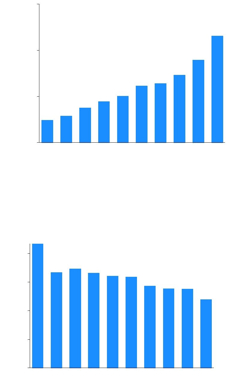
Figure 2 shows the distribution of the PIT revenue by income decile. Total revenue,
amounting to €65.1 billion, is very unevenly distributed, as expected from a progressive tax.
The first three deciles barely contribute to tax revenue, while the top 10% accounts for more
than half of it.
Figure 3 displays the average effective tax rates by income decile, that is, the ratio of
tax liabilities minus tax credits to gross income net of some deductions (base imponible). We
use this variable in the denominator because we do not observe gross income from some
income sources, such as self-employment income. Also, note that taxpayers whose tax
liabilities are negative are assigned a zero tax rate. As can be observed, the mean average
effective tax rates increase with income.
6
The bottom 30% of taxpayers face rates of virtually
0%, while tax rates for the well-off are around 24%, on average.
6 Average tax rates in respect of (observed) gross income are, on average, around two percentage points higher for
deciles 4 to 10 and 0.1 percentage points higher for deciles 1 to 3.
PIT REVENUE BY INCOME DECILE (2015) FIGURE 2
SOURCE: BdE PIT Microsimulation Model.
-118
-127
-115
447
1,677
2,958
4,905
7,587
11,779
36,066
0 10,000 20,000 30,000 40,000
Million euros
12345678910

BANCO DE ESPAÑA 17 DOCUMENTO OCASIONAL N.º 1707
2.3 Simulation example
In this section, we illustrate the outcome produced by the BdE PIT Microsimulation Tool by
simulating a hypothetical reform that should not be considered to be proposed by the
Banco de España. This consists of converting the tax benefit stemming from contributions
to private pension plans from a tax deduction (subtracted from the tax base, the current
situation or baseline scenario) to a (non-refundable) tax credit (subtracted from tax liabilities,
the reform scenario).
Under the 2015 legislation, the contributions made by taxpayers to private pension
plans could be deducted from the tax base, with limits set at €8,000 or €2,500 when the plan’s
beneficiary is herself or her spouse, respectively. The reform we simulate, instead applies this
tax benefit directly to tax liabilities, which cannot turn negative as a result (non-refundable tax
credit). We set the amount of the tax credit in order to roughly generate a revenue-neutral
reform. Specifically, the maximum amounts are set at €600 for contributions to own pension
plans and €300 for contributions to a spouse’s pension plan.
As a result of this hypothetical reform, set out for the purposes of illustration, we
estimate that total revenue would decrease by €68 million, the well-off being the hardest-hit on
aggregate (see Figure 4).
7
The aggregate tax liabilities of the bottom 30% would hardly change,
since the incidence of this tax benefit on this part of the income distribution is very low. The tax
revenue raised from deciles 4 to 9 would decrease by around €480 million, which would be
partially offset by an increase in the tax raised from the top decile.
7 Note that this reform does not affect withholdings. Policy actions that do change them would entail an additional
change in revenue from individuals whose income is withheld at source but who do not file a tax return.
MEAN AVERAGE EFFECTIVE TAX RATE BY INCOME DECILE (2015) FIGURE 3
SOURCE: BdE PIT Microsimulation Model.
0.55
0.02
0.23
3.15
6.67
8.94
11.83
14.56
17.62
23.93
0 5 10 15 20 25
%
12345678910

BANCO DE ESPAÑA 18 DOCUMENTO OCASIONAL N.º 1707
Figure 5 shows the percentage of winners and losers by income decile, while Table 3
summarises the quantitative effects of the reform. From deciles 4 to 9 almost all taxpayers are
better off, while in the top decile those affected by the reform are roughly evenly split between
winners and losers. Note that winners are those whose tax liabilities decrease as a result of the
tax change, while losers are those whose tax liabilities increase.
8
On average, winners in deciles
5 to 10 pay around €300 less in taxes while losers in the top decile face an increase of around
€1,500 in tax liabilities.
8 Tax increases and decreases are defined to occur when tax liabilities change by more than €1 or 0.001%.
REVENUE CHANGE BY INCOME DECILE FIGURE 4
SOURCE: BdE PIT Microsimulation Model
413
-115
-105
-90
-82
-59
-28
-1
-0
-0
-100 0 100 200 300 400
Million euros
10
9
8
7
6
5
4
3
2
1

BANCO DE ESPAÑA 19 DOCUMENTO OCASIONAL N.º 1707
Table 3 presents the numbers behind Figure 5, including the number of individuals
in each category for each income decile, as well as the total and average revenue change
within each category and decile.
PERCENTAGE OF WINNERS AND LOSERS BY INCOME DECILE FIGURE 5
SOURCE: BdE PIT Microsimulation Model.
WINNERS AND LOSERS TABLE 3
Total Winners Losers Neutral
Deciles Population
Gain (+) or
loss (-)
Avg. gain or
loss
Number % Avg. gain Number % Avg loss Number %
millions million € € millions € millions € millions
1 1.9 0 0.0 0.0 0.0 546.9 0.0 0.0 0.0 1.9 100.0
2 1.9 0 0.0 0.0 0.0 463.9 0.0 0.0 0.0 1.9 100.0
3 1.9 1 0.5 0.0 0.5 89.8 0.0 0.0 0.0 1.9 99.5
4 1.9 28 14.5 0.1 5.3 275.1 0.0 0.0 119.6 1.8 94.6
5 1.9 59 30.1 0.2 8.9 338.7 0.0 0.1 148.5 1.8 91.0
6 1.9 82 42.3 0.2 12.3 346.9 0.0 0.3 160.0 1.7 87.4
7 1.9 90 46.2 0.3 14.1 343.7 0.0 0.7 357.8 1.7 85.2
8 1.9 105 54.0 0.3 17.6 339.9 0.0 1.3 473.3 1.6 81.1
9 1.9 115 59.3 0.4 22.1 339.8 0.1 3.3 483.7 1.5 74.6
10 1.9 -413 -212.2 0.5 25.3 320.0 0.4 19.5 1,506.7 1.1 55.3
Total 19.5 68 3.5 2.1 10.6 333.8 0.5 2.5 1,266.9 16.9 86.9
SOURCE: BdE PIT Microsimulation Model.
0 20 40 60 80 100
%
12345678910
Winners Losers Neutral

BANCO DE ESPAÑA 20 DOCUMENTO OCASIONAL N.º 1707
Figure 6 shows the change in the (mean) average tax rate by income decile. The top
decile experiences a 0.2 percentage point increase in average tax rates, while the 8th decile
undergoes a similar effect of the opposite sign. The average tax rates of deciles 5 to 7 diminish
by slightly more than 0.2 percentage points.
Table 4 shows different measures of inequality of after-tax income before and after the
reform. Since the worse-off are concentrated in the well-off group, the Gini coefficient slightly
decreases. However, most of the other inequality indices increase, especially the 50/10 and the
75/25 ratios, since there is a non-negligible amount of winners concentrated in the middle of
the income distribution. It is worth noting nevertheless that the changes in the inequality indices
are rather small.
9
9 The model produces additional outputs, such as histograms of after-tax income and Lorenz curves. Moreover, it
allows the effects of the reform to be simulated by age group, rather than by income decile. These outputs are not
presented for space considerations.
CHANGE IN THE EFFECTIVE AVERAGE TAX RATE BY INCOME DECILE FIGURE 6
SOURCE: BdE PIT Microsimulation Model.
0.20
-0.17
-0.20
-0.21
-0.23
-0.21
-0.14
-0.01
-0.00
-0.00
-0.2 -0.1 0.0 0.1 0.2
Percentage Points
10
9
8
7
6
5
4
3
2
1

BANCO DE ESPAÑA 21 DOCUMENTO OCASIONAL N.º 1707
MEASURES OF INEQUALITY OF AFTER-TAX INCOME TABLE 4
Indices Pre-Reform Post-Reform Change (pp)
90/10 6.3 6.3 0.0014
90/50 2.1 2.1 -0.0034
50/10 3.1 3.1 0.0057
75/25 2.4 2.5 0.0039
75/50 1.5 1.5 0.0001
50/25 1.6 1.6 0.0025
Gini 0.38 0.38 -0.0007
SOURCE: BdE PIT Microsimulation Model.

BANCO DE ESPAÑA 22 DOCUMENTO OCASIONAL N.º 1707
3 The Banco de España Indirect Tax Microsimulation Model
This section introduces the microsimulation tool that calculates the Spanish VAT and excise
duties (IVA and impuestos especiales). The tool allows for changes in VAT on up to
119 different non-durable goods and for changes in the excise duties levied on four goods.
These reforms can be implemented jointly, which is especially useful, since, in the case of
goods subject to both VAT and excise duties, these taxes interact with each other. The tool
allows for morning-after effects of reforms, but it can also simulate hypothetical reforms taking
into account households’ behavioural reaction to price changes, given a level of expenditure on
non-durable goods, through the parameters estimated for a complete demand system.
3.1 The data
The main data used for this microsimulation tool are obtained from the Spanish Household
Expenditure Survey (Encuesta de Presupuestos Familiares, EPF). The sample contains 22,000
households per year with information on household expenditure for 255 commodities,
accounting for 78% of the expenditure according to the National Accounts in 2015. The
dataset also includes a large set of socio-demographic variables. The month in which
the survey was answered can be observed,
10
which allows the expenditure of each household
to be linked to the monthly prices for a particular commodity. The interviews of households are
uniformly distributed across each year.
In particular, the most recent wave of the survey is used for simulation purposes
(2015), and the pooled cross-sectional sample of the years 2006-2015 is used to estimate the
coefficients of the demand system. The sample contains a total of 217,000 observations.
The aggregation of goods into expenditure groups for the demand system is mainly driven by
heterogeneity among goods but also by the structure of Spanish indirect taxation. Each good
subject to excise duties is maintained as a separate group in the system (with the exception of
electricity) but is estimated jointly with the other groups of goods.
The second dataset used is the Spanish Consumer Price Index (Índice de Precios del
Consumo, IPC) containing monthly time series of price indices at national and regional level.
For the estimation of the demand system, monthly price indices by region (comunidad
autónoma) are used to obtain as much variation in prices as possible. In this case, the prices
are disaggregated into 37 goods, which are then aggregated into the 13 expenditure groups of
the demand system (described below). Official price indices assume a common consumption
basket across regions and therefore take the same value in the base year (2005). To correct for
this, a factor is applied to account for differences in price levels across regions, using the
estimations of Costa et al. (2015) for 2012. Hence, there are 17 x 10 x 12 (regions x years
x months) different prices for each commodity (i.e. 2,040).
For the simulation, the 2015 price index at national level is used, which offers a greater
disaggregation, into 119 prices.
11
These are the goods for which the microsimulator can
simulate changes in tax rates (VAT and excise duties if applicable).
10 This information was obtained under a special request to the Spanish Statistical Office (www.ine.es).
11 The initial disaggregation has 126 goods but some of them are combined due to interruptions and changes in the
series.

BANCO DE ESPAÑA 23 DOCUMENTO OCASIONAL N.º 1707
3.2 Framework of the Banco de España Indirect Taxation Microsimulation Model
The indirect taxation microsimulation model calculates the VAT and excise duties paid by each
household. It allows for the behavioural reactions of households to changes in prices arising
from taxation. Therefore, in addition to first-round or morning-after effects (changes in prices
and tax revenue resulting from changes in taxes keeping each household’s expenditure
constant for each commodity) we can estimate second-round effects arising from demand
adjustments. This adjustment is allowed in the form of substitution between commodities,
subject to a constant total level of consumption of non-durable goods. The model can
therefore be used for analyses such as running a simulation using the current VAT and excise
duty legislation to predict tax liabilities and revenues, making comparisons with hypothetical
reforms of the tax legislation (VAT or excise duty rates), and calculating welfare changes.
3.2.1 THE VALUE ADDED TAX AND EXCISE DUTIES
VAT is basically a tax on consumption expenditure. All sales are taxed, but registered traders
are allowed to deduct the tax charged on their inputs, so that the tax is effectively levied on the
value added at each stage of the production process. The only VAT that cannot be reclaimed is
that charged to the final purchaser and, therefore, only final consumption is taxed. Producers
can assume part of the increase in prices arising from a tax reform and this can be accounted
for in the simulations. A complete pass-through is usually assumed, except when the aim is to
obtain the short-run effects of reforms. In any case, the sensitivity of simulations to different
rates of pass-through can also be analysed.
Given the way in which VAT functions, the microsimulation model calculates
households’ tax liabilities for each good consumed before and after a reform. To simulate tax
reforms, the tax rates under the current legislation are deducted from the prices, and then the
new tax rates are added to obtain new prices. The demand system uses these new prices to
predict new shares of consumption of the different goods, allowing for substitution between
non-durable goods subject to a given total level of expenditure. As a result, the tax liabilities
paid by each household after the reform are obtained, having accounted for behavioural
responses to price changes.
3.2.2 PARAMETERS
Three types of parameters are used. First, the VAT tax rates that apply to each of the
119 goods of the national price index disaggregation. Second, 19 parameters that define the
different excise duties applied to the four goods subject to excise duties. Finally, the model
uses the behavioural parameters estimated by the demand system, explained in Section 3.2.3.
VAT Parameters
The VAT parameters for the 2015 legislation can take four different values, corresponding to
the four different tax rates existing: exempt (0%), super-reduced (4%), reduced (10%), and
standard (21%). A list of the 119 goods considered in the microsimulator and their
corresponding VAT tax rate in 2015 is shown in Table 5.
12
These are the goods for which we
can simulate a reform of the VAT rate.
12 For groups of goods taxed at different tax rates, a weighted average has been calculated using the price weights from
the IPC.

BANCO DE ESPAÑA 24 DOCUMENTO OCASIONAL N.º 1707
Good VAT Good VAT Good VAT Good VAT
Arroz 10 Alimentos para bebé 10 Aparatos de calefacción y de aire
acondicionado
21 Soporte para el registro de imagen y
sonido
21
Pan 4 Café, cacao e infusiones 10 Otros electrodomésticos 21 Juegos y juguetes 21
Pasta alimenticia 10 Agua mineral, refrescos y zumos 10 Reparación de electrodomésticos 21 Grandes equipos deportivos 21
Pastelería, bollería y masas cocinadas 10 Espirituosos y licores 21 Cristalería, vajilla y cubertería 21 Otros artículos recreativos y deportivos 21
Harinas y cereales 4 Vinos 21 Otros utensilios de cocina y menaje 21 Floristería y mascotas 15.5
Carne de vacuno 10 Cerveza 21 Herramientas y accesorios para casa y
jardín
21 Servicios recreativos y deportivos 21
Carne de porcino 10 Tabaco 21 Artículos de limpieza para el hogar 21 Servicios culturales 21
Carne de ovino 10 Prendas exteriores de hombre 21 Otros artículos no duraderos para el
hogar
21 Libros de entretenimiento y de texto 4
Carne de ave 10 Prendas interiores de hombre 21 Servicio doméstico y otros servicios
para el hogar
21 Prensa y revistas 4
Charcutería 10 Prendas exteriores de mujer 21 Medicamentos y otros productos
farmacéuticos
4 Material de papelería 21
Preparados de carne 10 Prendas interiores de mujer 21 Material terapéutico 21 Viaje organizado 10
Otras carnes y casquería 10 Prendas de vestir de niño y bebé 21 Servicios médicos y paramédicos no
hospitalarios
21 Educación Infantil 0
Pescado 10 Complementos y reparación y limpieza
de prendas de vestir
21 Servicios dentales 0 Enseñanza obligatoria 0
Crustáceos y moluscos 10 Calzado de hombre 21 Servicios hospitalarios 0 Bachillerato 0
Pescado en conserva y preparados 10 Calzado de mujer 21 Automóviles 21 Enseñanza superior 0
Leche 4 Calzado de niño y bebé 21 Otros vehículos 21 Otras enseñanzas 0
Otros productos lácteos 10 Reparación de calzado 21 Repuestos y accesorios de
mantenimiento
21 Restaurantes, bares y cafeterías y
Cantinas
10
Quesos 4 Alquiler de vivienda 0 Carburantes y lubricantes 21 Hoteles y otros alojamientos 10
Huevos 4 Materiales para la conservación de la
vivienda
10 Servicios de mantenimiento y
reparaciones
21 Servicios para el cuidado personal 21
Mantequilla y margarina 10 Servicios para la conservación de la
vivienda
10 Otros servicios relativos a los vehículos 21 Artículos para el cuidado personal 21
Aceites 10 Distribución de agua 10 Transporte por ferrocarril 10 Joyería, bisutería y relojería 21
Frutas frescas 4 Recogida de basuras, alcantarillado y
otros
10 Transporte por carretera 10 Otros artículos de uso personal 21
Frutas en conserva y frutos secos 10 Electricidad 21 Transporte aéreo 10 Servicios sociales 0
Legumbres y hortalizas frescas 4 Gas 21 Otros servicios de transporte 10 Seguros para la vivienda 0
Legumbres y hortalizas secas 4 Otros combustibles 21 Servicios postales 0 Seguros médicos 0
Legumbres y hortalizas congeladas y
en conserva
4 Muebles 21 Equipos telefónicos 21 Seguros de automóvil 0
Patatas y sus preparados 4 Otros enseres 21 Servicios telefónicos 21 Otros seguros 0
Azúcar 10 Artículos textiles para el hogar 21 Equipos de imagen y sonido 21 Servicios financieros 0
Chocolates y confituras 10 Frigoríficos, lavadoras y lavavajillas 21 Equipos fotográficos y
cinematográficos
21 Otros servicios 21
Otros productos alimenticios 10 Cocinas y hornos 21 Equipos informáticos 21
Notice that these tax rates are the result of combining the different tax rates applicable to each good contained in each category.
SOURCE: Banco de España.
DISAGGREGATION OF GOODS CONSIDERED IN THE MICROSIMULATOR AND THEIR VAT RATES IN 2015
TABLE 5

BANCO DE ESPAÑA 25 DOCUMENTO OCASIONAL N.º 1707
Table 6 shows the evolution of VAT rates in Spain from 1986. It shows that every tax
reform implemented from 1986 onwards increased VAT, with the sole exception of the one
introduced in 1993.
Table 7 compares the VAT tax rates across the EU countries. VAT rate structures vary
widely within the EU. Most countries do not have a super-reduced rate (that is, a rate below
5%), however many of them have two reduced tax rates.
13
13 9% of the total consumption of the EPF derives from goods taxed at the super-reduced rate, 31.5% at the reduce
rate, 49.2% at the standard rate and 10.4% are exempt.
Dates Reduced Rate Standard Rate
01/01/1986 6 12
01/01/1992 6 13
01/08/1992 6 15
01/01/1993 3 | 6 15
01/01/1995 4 | 7 16
01/07/2010 4 | 8 18
01/09/2012 4 | 10 21
SOURCE: European Commission.
EVOLUTION OF VAT RATES IN SPAIN TABLE 6
VAT TAX RATES BY COUNTRY TABLE 7
Member State Code Super-reduced rate Reduced rate Standard rate
Belgium
BE - 6 / 12 21
Bulgaria BG - 9 20
Czech Republic CZ - 10 / 15 21
Denmark DK - - 25
Germany DE - 7 19
Estonia EE - 9 20
Ireland IE 4.8 9 / 13,5 23
Greece EL - 6 / 13 24
Spain ES 4 10 21
France FR 2.1 5,5 / 10 20
Croatia HR - 5 / 13 25
Italy IT 4 5 / 10 22
Cyprus CY - 5 / 9 19
Latvia LV - 12 21
Lithuania LT - 5 / 9 21
Luxembourg LU 3 8 17
Hungary HU - 5 / 18 27
Malta MT - 5 / 7 18
Netherlands NL - 6 21
Austria AT - 10 / 13 20
Poland PL - 5 / 8 23
Portugal PT - 6 / 13 23
Romania RO - 5 / 9 20
Slovenia SI - 9.5 22
Slovakia SK - 10 20
Finland FI - 10 /14 24
Sweden SE - 6 / 12 25
United Kingdom
UK - 5 20
SOURCE: European Commission.

BANCO DE ESPAÑA 26 DOCUMENTO OCASIONAL N.º 1707
Excise Duty Parameters
The excise duty legislation applies different taxes to each commodity. In particular, calculation
of the after-tax prices requires different types of taxes to be taken into account. Ad valorem tax
rates, like VAT tax rates, are charged as a percentage of the price. Ad quantum taxes, in
contrast, are calculated on the basis of the quantities of the good (according to the number of
cigarettes, litres of alcohol, etc.). Other excise duties considered are the Recargo de
Equivalencia (a percentage rate added to the VAT rate) and Comisión de Estanco (a retail
mark-up determined by law). The excise duties charged on each good considered are detailed
in Table 8.
SUMMARY OF GOODS SUBJECT TO EXCISE DUTIES TABLE 8
Expenditure
groups
Commodities
included
Taxes Value
Nominal market
price (a)
Tobacco
Cigarettes
Ad valorem (%) 0.51
€4.49
Ad quantum (€ per 20 cigarettes) 0.482
Recargo de equivalencia (%) 0.0175
Comisión Estanco (€) 0.09
Fine-cut
Ad valorem (%) 0.415
Ad quantum
(€ per 20 standardised cigarettes)
0.44
Recargo de equivalencia (%) 0.0175
Comisión Estanco (€) 0.085
Others
Ad valorem (%) 0.415
Ad quantum
(€ per 20 standardised cigarettes)
0.44
Recargo de equivalencia (%) 0.0175
Comisión Estanco (€) 0.085
Alcohol
Spirits
Ad quantum
(€ per litre of pure alcohol)
9.13 €12.29
Beer Ad quantum (€ per litre of beer) 0.09 €1.81
Vehicle fuels
Petrol
Estatal general
(ad quantum, cents per litre)
40.069
€122.83
Estatal especial
+ Autonómico especial
(ad quantum, cents per litre)
6.16
Diesel
Estatal general
(ad quantum, cents per liter)
30.7
€111.44
Estatal especial
+ Autonómico especial
(ad quantum, cents per litre)
6.27
Electricity Electricity Ad valorem (%) 5.11269632 €0.1526
SOURCE: Own calculations, based on Official State Gazette (BOE) and (a) AEAT annual report.

BANCO DE ESPAÑA
27
DOCUMENTO OCASIONAL N.º 1707
Because the price information is given in terms of price indices, for the simulation of ad
quantum taxes the average market price of the good concerned is needed as a starting point.
These prices are taken from the AEAT annual report, which reports average nominal prices for
each group of goods considered in this paper, as shown in the last column of Table 8. Then, all
the taxes are deducted from these market prices in order to obtain before-tax prices. Finally,
we calculate the new after-tax prices using the post-reform tax parameters. This procedure
allows us to calculate the percentage difference between before-tax and after-tax market
prices and to extrapolate it to the price index of the corresponding good.
Each group of goods subject to excise duties has its own specific features. Tobacco is
broken down into cigarettes (cigarrillos), fine-cut tobacco (picadura) and other tobacco (puros,
cigarritos …). The formula to calculate the after-tax price is the same for all three goods:
=
(+)∗(1++)
1−∗(1++)−
where is the after-tax price, is the before-tax price (the net-of-tax price), is the ad valorem
tax rate, is the ad quantum tax rate, is the Recargo de Equivalencia, is
the Comisión de Estanco, and is the VAT tax rate. The values of the excise duties, however,
are different for the three goods, therefore there are a total of 12 excise duty parameters that
can be changed in a simulation.
Excise duties on alcohol also differ according to the product, with spirits and beer
taxed at different rates.
14
The formula to apply these taxes is the same for both goods:
=
(
+∗ℎ
)
∗(1+)
where is the after-tax price, is the before-tax price (the net-of-tax price), is the ad
quantum tax rate per litre, ℎ is the share of pure alcohol per litre of spirit (on average), and is
the VAT tax rate.
For vehicle fuels, we distinguish between diesel (gasóleo) and petrol (gasolina), which
again are subject to different excise duties, but according to the same formula:
=
(
+++
)
∗(1+)
where is the after-tax price, is the before-tax price, is the State general tax rate, is the
State specific tax rate, is the regional specific tax rate, and is the VAT
tax rate. We consider the two specific tax rates ( and ) together, as reported by the AEAT.
For electricity, in addition to the VAT,, there is only one excise duty, the ad valorem
tax, , which is applied to the price using the formula:
15
=∗
(
1+
)
∗(1+)
14 Wine is not subject to any excise duties, but only to VAT at the regular rate of 21%.
15 The law provides for a minimum tax rate of 5.11%, but in most cases the tax rate resulting from the application of the
formula below is higher.

BANCO DE ESPAÑA 28 DOCUMENTO OCASIONAL N.º 1707
3.2.3 THE DEMAND SYSTEM: BEHAVIOUR IN THE BANCO DE ESPAÑA INDIRECT TAXATION
MICROSIMULATION MODEL
For the estimation of the behavioural parameters, we aggregate expenditure on the 255 goods
of the EPF into 13 groups of non-durable expenditure. We define a 14th group containing
durable expenditures, which is not included in the estimation of the demand system, but for
which total revenues are calculated. We try to group goods taking into account separability
conditions but also differences in their tax treatment. Goods subject to excise duties
(underlined below) are also included in the demand system. Notice that wine is not subject to
excise duties and electricity is included in the domestic utilities group because it has a share
that is too small for it to constitute a group on its own. The groups are:
1. Food and beverages: fresh and processed food and non-alcoholic drinks
2. Alcoholic drinks: spirits, beer and wine
3. Tobacco: cigarettes, fine-cut and others
4. Clothing and footwear: including repairs
5. Domestic utilities: water, electricity, gas, refuse collection
6. Household non-durables: including domestic services
7. Health: pharmaceutical products, dental and private medical services
8. Vehicle fuels: petrol and diesel
9. Transport: trains, buses, planes, taxis and related services
10. Communications: postal services and telephone services
11. Leisure and culture: cultural services, books, newspapers and package holidays
12. Hotels and restaurants: restaurants, hotels and other housing services
13. Other non-durables: personal care products and services, insurance and other
14. Durables: furniture and home appliances, cars, electronic equipment, private
education services and jewellery
The demand system consists of a set of 13 non-durable goods demand equations,
which are estimated jointly. We use the Quadratic Almost Ideal Demand System (QUAIDS)
introduced by Banks, Blundell, and Lewbel (1997) as an extension of the Almost Ideal Demand
System (AIDS) of Deaton and Muellbauer (1980). This is a useful demand system to evaluate
the welfare impact of tax reforms. The reason is that it allows the share of each good in total
expenditure to vary in a flexible way with respect to income and prices. In the case of income,
the good could be a luxury (elasticity greater than 1) at one level of expenditure and a necessity
(elasticity smaller than 1) at another level of expenditure. The model assumes that the utility
obtained from the consumption of any good is not affected by the labour supply of any
member of the household, except insofar as the estimated equations for each good can be
made conditional on labour supply variables.
Some goods have a high rate of zeroes because they are not consumed by the
households (not due to infrequency of purchase). For these we use a two-stage estimation
strategy. First, we estimate probit models for tobacco and domestic utilities as in equation (1).
=
+
(1)
where ℎ denotes household, is a subscript for goods ( = 1,…,), for time
( = 1,…,) and is a vector of socio-demographic variables. Then, we obtain the Mill’s
inverse probability ratios according to expressions (2) for consumers of good ( = tobacco,
vehicle fuels) and (3) for non-consumers:

BANCO DE ESPAÑA 29 DOCUMENTO OCASIONAL N.º 1707
=
(2)
=
(3)
The QUAIDS is estimated in the second stage, including the inverse Mill’s ratios as
regressors in all the equations. The demand system is based on the indirect utility function
presented in (4):
=
()
()
+()
(4)
where (), () and () are price indices defined as:
(
)
=
+
∑
+
∑∑
(5)
(
)
=
∏
(6)
(
)
=
∑
ln
(7)
where and both denote number of goods (, =1,…,). Maximising (4) subject to the
budget constraint, we can express the share of expenditure on each good , for each
household ℎ, in each period , as:
=
+
()
+
()
()
+
∑
(8)
We define
=
(
) as a function of a vector
containing a constant, socio-
demographic variables (
) and the inverse Mill’s ratio calculated in the first stage. In fact, this
involves modifying equation (5) accordingly, so that its inclusion gives rise to new adding-up
conditions that will be taken into account at the estimation stage. The resulting equation is:
(
)
=
+
∑
+
∑∑
(9)
To perform welfare analysis, we require the resulting demands to be consistent with
utility maximisation, thus satisfying theoretical adding-up, homogeneity, symmetry and
negativity restrictions. Adding-up is satisfied leaving aside one of the equations in the
estimation and homogeneity and symmetry are imposed at the estimation stage. Negativity
cannot be imposed but it can be tested for by looking at the Slustky matrix. All these
theoretical conditions limply the following linear restrictions on the parameters of the model:
Adding up:
∑
=1
;
∑
=0
;
∑
=0
for all j;
∑
=0
Homogeneity:
∑
=0
for all
Symmetry:
=
Once the model is estimated, we use the results to evaluate the impact of price
changes (following a tax reform) on consumer welfare. We do so using the associated

BANCO DE ESPAÑA 30 DOCUMENTO OCASIONAL N.º 1707
expenditure functions of the QUAIDS. We calculate the compensating variation CV. CV is
defined as the change in income a household would require to be indifferent between the
original prices and the new prices. So, if (.) is the expenditure function associated with
the model, the CV for household ℎ is:
=
(
∗
,
)
−
(
∗
,
)
(10)
∗
is the original value of utility for household ℎ,
is the price vector pre-reform and
is the
new price vector following the reform.
The results of the QUAIDS are summarised in the elasticities shown in Table 9 (shares
of expenditure, income and uncompensated own-price elasticities) and Table 10 (cross-price
elasticities). The income elasticities obtained are close to the results found in the literature using
Spanish data (Labeaga and López (1996), Labeaga and Puig (2003) or Christensen (2014)) and
even internationally (Banks, Blundell, and Lewbel (1997)). As expected, all income elasticities
are positive, and those for necessity goods such as food, domestic utilities and
communications have lower values, while those for leisure, household non-durables, and health
have the highest values. Food, tobacco, domestic utilities and communications are necessities
while clothing and footwear, household non-durables, health, leisure and culture, hotels and
restaurants and other non-durables are luxury goods. We cannot reject a unitary elasticity for
alcoholic drinks, vehicle fuels and transport. The result for health can be explained because the
survey only collects information on private expenditure on this good. Uncompensated own-
price elasticities are all negative at average values of the variables, as expected. The most
elastic goods are leisure and culture, household non-durables, transport and clothing and
footwear, while food and beverages at home are not sensitive to price changes.
OBSERVED (2015) AND PREDICTED SHARES, INCOME AND OWN-PRICE ELASTICITIES TABLE 9
Observed
shares
Predicted
shares
Income
elasticity
Uncompensated
own-price elasticity
1. Food and beverages 0.2775 0.2766 0.715*** -0.109
2. Alcoholic drinks 0.0106 0.0114 1.010*** -0.993***
3. Tobacco 0.0219 0.0221 0.846*** -0.833***
4. Clothing and footwear 0.0739 0.0759 1.385*** -1.011***
5. Domestic utilities 0.1370 0.1362 0.538*** -0.525***
6. Household non-durables 0.0402 0.0433 1.548*** -1.969***
7. Health 0.0382 0.0354 1.901*** -0.524***
8. Vehicle fuels 0.0635 0.0652 0.973*** -0.159***
9. Transport 0.0522 0.0520 0.955*** -1.090***
10. Communications 0.0511 0.0479 0.592*** -0.189***
11. Leisure and culture 0.0476 0.0478 1.421*** -2.253***
12. Hotels and restaurants 0.1254 0.1234 1.404*** -0.974***
13. Other non-durables 0.0607 0.0638 1.224*** -0.572*
* p<0.05, **p<0.01, ***p<0.001
SOURCE: BdE VAT Microsimulation Model.

BANCO DE ESPAÑA 31 DOCUMENTO OCASIONAL N.º 1707
CROSS-PRICE ELASTICITIES TABLE 10
1.
Food and
beverages
2.
Alcoholics
drinks
3.
Tobacco
4.
Clothing
and
footwear
5.
Domestic
utilities
6.
Household
non-durables
7.
Health
8.
Vehicle fuels
9.
Transport
10.
Communications
11.
Leisure
and
culture
12.
Hotels
and
restaurants
13.
Other
non-durables
1. Food and beverages -0.109 0.02 -0.009 0.181*** 0.216*** -0.079 -0.179*** -0.224*** -0.142** 0.091** 0.170*** -0.379*** -0.272**
2. Alcoholic drinks 0.487 -0.993*** 0.104 0.256*** 0.715*** -1.959*** -0.281* -0.806*** 0.711*** 0.422** 1.852*** -0.874* -0.645
3. Tobacco -0.14 0.046 -0.833*** -0.364*** -0.106 0.456 0.556*** -0.027 0.188 0.427*** 0.117 -0.61 -0.556
4. Clothing and footwear 0.449* 0.029 -0.120* -1.011*** -0.404*** 0.076 0.042 -0.158** 0.007 -0.053 0.16 -0.462* 0.061
5. Domestic utilities 0.576*** 0.067 -0.014 -0.210*** -0.525*** 0.118 -0.577*** 0.046 0.062 -0.019 0.056 -0.377*** 0.258*
6. Household non-durables -0.784* -0.489 0.246** 0.135* 0.216 -1.969*** 0.944*** -0.176* -0.058 0.307* -1.013*** 1.468*** -0.375
7. Health -1.998*** -0.102 0.405*** 0.068 -2.356*** 1.255*** -0.524*** 1.320*** 0.253 -1.200*** 0.026 -0.252 1.203*
8. Vehicle fuels -0.925*** -0.109 -0.012 -0.136*** 0.021 -0.073 0.569*** -0.159*** -0.032 -0.145* -0.232* 0.272 -0.011
9. Transport -0.854*** 0.141 0.084 0.046 0.092 -0.022 0.180** -0.045 -1.090*** 0.210** 0.480*** -0.191 0.016
10. Communications 0.522*** 0.085 0.197*** -0.015 -0.047 0.277* -0.651*** -0.176*** 0.222** -0.189*** 0.046 -0.334** -0.530***
11. Leisure and culture 0.746*** 0.366 0.041 0.249*** 0.025 -0.816*** 0.03 -0.375*** 0.461*** 0.004 -2.253*** 1.196*** -1.095***
12. Hotels and restaurants -1.069*** -0.076 -0.131** -0.302*** -0.458*** 0.496*** -0.047 0.132** -0.103 -0.187** 0.494*** -0.974*** 0.823***
13. Other non-durables -1.594*** -0.125 -0.257*** 0.105** 0.486*** -0.277 0.713*** -0.034 0.002 -0.563*** -1.036*** 1.929*** -0.572*
* p<0.05, **p<0.01, ***p<0.001
SOURCE: BdE VAT Microsimulation Model.

BANCO DE ESPAÑA 32 DOCUMENTO OCASIONAL N.º 1707
3.2.4 THE OUTPUT OF THE MODEL
The model simulates the tax paid by each household (including both VAT and excise duties)
depending on its choice of consumption basket. Then, it computes and aggregates certain variables
either by income decile or by age group in order to perform some comparisons. The variables of
interest analysed are similar to those analysed in the case of the microsimulator of direct taxation:
total revenue, average tax rates, winners and losers, and several inequality measures such as the
distribution of after-tax income, Lorenz curve, Gini coefficient and some percentile ratios.
Since the microsimulator of indirect taxation allows for the behavioural responses of
households, the output of the model also includes a measure of the welfare impact of the
reform, calculated as the compensating variation for each household, that is to say
the monetary amount that a household should receive or pay to maintain its pre-reform utility in
annual terms.
16
The utility function assumed is based on Banks, Blundell, and Lewbel (1997).
Section 3.3 shows this output for two simulation exercises: first, for a change in the
VAT rate and second, for a change in excise duties.
3.2.5 THE ACCURACY OF THE MODEL
The total household expenditure on taxable goods (that is, excluding goods without price such as
narcotics or imputed rents, and goods exempt of VAT such as financial products) represented in
our dataset amounts to €350,762 million, while the AEAT reports a household expenditure on
taxable goods of €331,361 million. Our current model predicts €59,062 million of household VAT
revenues and excise duties for 2015, while the revenues reported by the AEAT amount to
€71,175 million. This difference (17.02%) could arise from the following factors. First, expenditure
measurement and reporting errors (under-reporting in the case of tobacco; infrequency of
purchase of leisure goods, for example; and individuals not represented in the survey like those in
prison, hospital, etc.). Second, and in the opposite direction, tax evasion, which could affect
expenditure on some services, maintenance, etc. And third, minor errors incurred during the
aggregation of goods into 119 groups using available price data.
The results could be adjusted to improve the prediction of total aggregated revenue.
However, since we are also interested in the distributional effects of the reform we chose not to
make these adjustments.
17
3.2.6 BASELINE RESULTS: INDIRECT TAX REVENUES AND THE DISTRIBUTION OF TAX LIABILITIES
UNDER THE 2015 LEGISLATION
Figure 7 shows the revenue that the microsimulator predicts under the existing VAT and excise
duty legislation, disaggregated by income deciles.
18
The total revenue amounts to €59,062 million.
16 Note that, under this definition, a reform that increases a household’s welfare leads to a negative compensating
variation (the amount this household should pay back to return to its initial utility level). The output produced by the
model, however, shows the welfare gain, and therefore such a reform leads to a positive value (an increase in welfare).
17 Sources of adjustment that could be used include: Data on total consumption of vehicle fuels (except in the case of tax
evasion) provided by the Comisión Nacional de Mercados y Competencia. Data from the Comisionado de Tabacos for
tobacco, and from the Asociación de Fabricantes de Bebidas Espirituosas, Cerveceros de España and the Federación
Española del Vino for spirits, beer and wine, respectively.
18 We show the output of the microsimulator in terms joint VAT and excise duties given that each tax depends from one
another (c.f. formulae in Sectiorn 2.2.2). A microsimulator of VAT alone causes a downward bias in the estimated
baseline revenue because this amount is calculated simulating the elimination of all excise duties, and such a reform also
impacts VAT revenue downwards. Nonetheless, we have computed the total revenues and the average effective tax rate
without excise duties as a robustness check. Total revenues amounts to €45,707 million, which is an 88.93% of the VAT
revenue reported by the AEAT, and average tax rate is 11.88%, close to the one reported by Laborda et al (2016) and
Laborda et al (2017).
BANCO DE ESPAÑA 33 DOCUMENTO OCASIONAL N.º 1707
Figure 8 presents the average tax rate faced by each income decile calculated as a
percentage of income. That is, the total tax payments as a percentage of income. The tax rates in
this case decrease over the income deciles, showing that the VAT-excise duties tax is regressive.
REVENUE FROM VAT AND EXCISE DUTIES BY INCOME DECILE IN 2015 FIGURE 7
SOURCE: BdE VAT Microsimulation Model.
MEAN OF AVERAGE EFFECTIVE TAX RATE (AS % OF INCOME)
BY INCOME DECILE
FIGURE 8
SOURCE: BdE VAT Microsimulation Model.
2,441
2,900
3,774
4,462
5,038
6,158
6,418
7,340
8,958
11,573
0
5,000
10,000
15,000
Million euros
12345678910
VAT
and
Excise
Duties
Revenue
by
Income
Decile
21.69
16.71
17.33
16.61
16.08
15.92
14.37
13.85
13.82
11.99
0
5
10
15
20
12345678910

BANCO DE ESPAÑA 34 DOCUMENTO OCASIONAL N.º 1707
However, Figure 9 presents the average tax rate faced by each income decile
calculated as a percentage of consumption.
19
That is, the total tax payments as a percentage
of consumption. In this case, the tax rates are mildly flat.
The disparity in the results when the effective tax rate is computed relative to income
and relative to consumption is not new in the literature. When looking at VAT payments as a
percentage of total expenditure (as opposed to disposable income), Figari and Paulus (2012)
conclude that for five European countries (Belgium, Greece, Ireland, Hungary and the UK), the
VAT system does not seem to be regressive. Indeed, households in the richest disposable
income decile pay a higher fraction of their total expenditure on VAT than households in the
lowest income decile because they spend a higher proportion of their expenditure on goods
and services that are taxed at higher rates.
20
Given that the European Directive (2006/112/EC) of 28 November 2006 defines VAT
as “a general tax on consumption proportional to the price of the goods and services” the tax
base is the individual expenditure instead of individual income as in the PIT Microsimulation
model. Therefore, from now on, we provide average tax rates computed as a percentage of
consumption instead of income.
21
19 Notice that the denominator includes consumption on goods exempt from VAT or excise duties as is usual in the literature.
20 From a theoretical point of view, redistributing income through income tax is less costly in efficiency terms,
because it does not distort individual consumption (Atkinson and Stiglitz, 1976; Mankiw et al., 2009). That is, if the
policy objective is to tax individuals on the basis of their income, it is preferable to tax income directly, unless
consumption choices reveal something about income that cannot be captured by personal income tax (e.g. there
is significant tax evasion and under-reporting that hinders the efficient collection of income tax, and consumption
tax is less prone to evasion).
21 The IFS report for the European Commission also reports the average tax rates as a percentage of consumption when
evaluating reforms. (Adam et al., 2011).
MEAN OF AVERAGE EFFECTIVE TAX RATE (AS % OF CONSUMPTION)
BY INCOME DECILE IN 2015
FIGURE 9
SOURCE: BdE VAT Microsimulation Model.
15.22
14.78
15.15
15.40
15.36
15.60
15.64
15.71
15.82
15.57
0
5
10
15
20
25
12345678910
Mean
of
Average
Tax
Rate
(over
consumption)
by
Income
Decile

BANCO DE ESPAÑA 35 DOCUMENTO OCASIONAL N.º 1707
3.3 Simulation examples
In what follows we present two hypothetical reforms to illustrate the possibilities of the BdE VAT
Microsimulation Tool. These examples should not be understood in any way as reform
proposals of the Banco de España.
3.3.1 A CHANGE IN VAT: A ONE POINT INCREASE IN THE STANDARD VAT RATE
In the first illustrative example of the BdE VAT Microsimulation Tool we simulate a one point
increase in the VAT rate for goods taxed under the standard rate, from 21% to 22%.
Figure 10 shows the revenue change as a result of the reform, disaggregated by
income decile. The total revenue increases by €1,317 million. Revenue increases more in
the top deciles given that the richest households consume more goods and services than the
poorest one.
Figure 11 shows the winners and losers of the reform, as measured by their tax
payments. Since almost every household consumes goods taxed at the standard VAT rate,
every household loses.
REVENUE CHANGE BY INCOME DECILE FIGURE 10
SOURCE: BdE VAT Microsimulation Model.
269
201
164
142
136
111
97
82
63
52
0 100 200 300
Million euros
10
9
8
7
6
5
4
3
2
1

BANCO DE ESPAÑA 36 DOCUMENTO OCASIONAL N.º 1707
Table 11 shows the amounts behind Figure 11. For example, we can see that, among
all losers, the average loss is €72.0. Losers belonging to the bottom percentile lose €28.8 on
average, while losers belonging to the top percentile lose €147.9 on average.
Figure 12 shows that the average tax rate (as a percentage of consumption) of the
upper deciles increases most, as is to be expected from the fact that richer households spend
a larger share of their total expenditure on goods taxed at the standard rate than poorer ones.
WINNERS AND LOSERS FIGURE 11
SOURCE: BdE VAT Microsimulation Model
WINNERS AND LOSERS TABLE 11
Total Winners Losers Neutral
Deciles Population
Gain (+) or
loss (-)
Avg. gain
or loss
Number % Avg. gain Number % Avg loss Number %
millions million € € millions € millions € millions
1 1.8 -52 -28.5 0.0 0.0 0.0 1.8 99.0 28.8 0.0 1.0
2 1.8 -63 -34.3 0.0 0.0 0.0 1.8 100.0 34.3 0.0 0.0
3 1.8 -82 -45.1 0.0 0.0 0.0 1.8 100.0 45.1 0.0 0.0
4 1.8 -97 -53.2 0.0 0.0 0.0 1.8 100.0 53.2 0.0 0.0
5 1.8 -111 -60.6 0.0 0.0 0.0 1.8 100.0 60.6 0.0 0.0
6 1.9 -136 -73.1 0.0 0.0 0.0 1.9 100.0 73.1 0.0 0.0
7 1.8 -142 -79.0 0.0 0.0 0.0 1.8 100.0 79.0 0.0 0.0
8 1.8 -164 -89.1 0.0 0.0 0.0 1.8 100.0 89.1 0.0 0.0
9 1.8 -201 -109.4 0.0 0.0 0.0 1.8 100.0 109.4 0.0 0.0
10 1.8 -269 -147.9 0.0 0.0 0.0 1.8 100.0 147.9 0.0 0.0
Total 18.3 -1,317 -72.0 0.0 0.0 0.0 18.3 99.9 72.0 0.0 0.1
SOURCE: BdE VAT Microsimulation Model.
0 .2 .4 .6 .8 1
12345678910
yy
Winners Losers Neutrals

BANCO DE ESPAÑA 37 DOCUMENTO OCASIONAL N.º 1707
With regard to welfare changes, Figure 13 shows that all deciles of income experience
a welfare reduction, which is larger for the top deciles. The welfare change is measured using
the compensating variation, as explained in Sections 3.2.3 and 3.2.4. In particular, the annual
income of the households in the top decile would need to increase by €151.49 in order to
restore their initial utility level.
CHANGE IN AVERAGE TAX RATE (AS % OF CONSUMPTION) BY
INCOME DECILE
FIGURE 12
Source: BdE VAT Microsimulation Model
WELFARE CHANGE FIGURE 13
SOURCE: BdE VAT Microsimulation Model.
0.35
0.35
0.34
0.34
0.34
0.33
0.33
0.33
0.32
0.32
0 .1 .2 .3 .4
Percentage points
10
9
8
7
6
5
4
3
2
1
Change
in
VAT
Excise
Duties
Rate
(over
consumption)
by
Income
Decile
-151.49
-116.06
-96.45
-87.07
-81.25
-70.07
-62.42
-54.18
-42.80
-34.90
-150 -100 -50 0
euros
10
9
8
7
6
5
4
3
2
1

BANCO DE ESPAÑA 38 DOCUMENTO OCASIONAL N.º 1707
Table 12 shows the effect of the reform on inequality, which in this case is a very
small decrease in the Gini coefficient. Looking at the percentile ratios, we observe a moderate
decrease in inequality in all percentile ratios except for 50/25.
3.3.2 A CHANGE IN EXCISE DUTIES: AN INCREASE IN THE AD QUANTUM TAX ON SPIRITS
In this second illustrative example we simulate an increase in the ad quantum tax on spirits
from €9.13 per litre of pure alcohol to €17.94, which is the average tax rate in the euro area
and close to that in France.
Figure 14 shows the effect on tax revenue from each decile, the total increase
amounting to €145 million.
INEQUALITY MEASURES: AFTER-TAX CONSUMPTION TABLE 12
Indices Pre-Reform Post-Reform Change (pp)
90/10 6.027 6.024 -0.0026
90/50 2.298 2.297 -0.0007
50/10 2.622 2.622 -0.0004
75/25 2.558 2.557 -0.0015
75/50 1.569 1.568 -0.0010
50/25 1.630 1.630 0.0001
Gini 0.363 0.363 -0.00013
SOURCE: BdE VAT Microsimulation Model.
REVENUE CHANGE BY INCOME DECILE FIGURE 14
SOURCE: BdE VAT Microsimulation Model.
26
20
17
16
16
13
12
10
8
6
0 5 10 15 20 25
Million euros
10
9
8
7
6
5
4
3
2
1
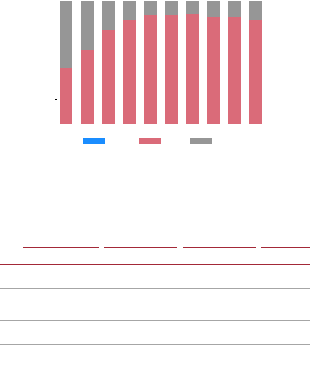
BANCO DE ESPAÑA 39 DOCUMENTO OCASIONAL N.º 1707
In Figure 15 we observe that for each decile there is a significant proportion of
households that are neutrals with regard to the reform. This result is explained by the high
proportion of households with zero spirit expenditure in their budgets (close to 30% on
average). The proportion of losers is higher for the middle deciles.
Table 13 provides a more detailed view of the effect of the reform. In total, 79.4% of
households lose, while the remaining 20.6% are neutrals. The average loss among all losers is
€7.9. Bottom decile losers experience an average loss of €3.5 while top decile losers
experience an average loss of €14.2.
WINNERS AND LOSERS FIGURE 15
SOURCE: BdE VAT Microsimulation Model.
WINNERS AND LOSERS TABLE 13
Total Winners Losers Neutral
Deciles Population
Gain (+) or
loss (-)
Avg. gain
or loss
Number % Avg. gain Number % Avg loss Number %
millions million € € millions € millions € millions
1 1.8 -6 -3.5 0.0 0.0 0.0 0.8 46.0 5.6 1.0 54.0
2 1.8 -8 -4.3 0.0 0.0 0.0 1.1 60.2 5.7 0.7 39.8
3 1.8 -10 -5.6 0.0 0.0 0.0 1.4 76.6 6.6 0.4 23.4
4 1.8 -12 -6.4 0.0 0.0 0.0 1.5 84.6 7.0 0.3 15.4
5 1.8 -13 -7.3 0.0 0.0 0.0 1.6 89.0 7.8 0.2 11.0
6 1.9 -16 -8.4 0.0 0.0 0.0 1.7 88.7 8.8 0.2 11.3
7 1.8 -16 -8.8 0.0 0.0 0.0 1.6 89.6 9.2 0.2 10.4
8 1.8 -17 -9.4 0.0 0.0 0.0 1.6 87.1 9.9 0.2 12.9
9 1.8 -20 -11.1 0.0 0.0 0.0 1.6 87.0 11.6 0.2 13.0
10 1.8 -26 -14.2 0.0 0.0 0.0 1.5 85.1 15.0 0.3 14.9
Total 18.3 -145 -7.9 0.0 0.0 0.0 14.5 79.4 9.0 3.8 20.6
SOURCE: BdE VAT Microsimulation Model.
0 .2 .4 .6 .8 1
12345678910
yy
Winners Losers Neutrals

BANCO DE ESPAÑA 40 DOCUMENTO OCASIONAL N.º 1707
Figure 16 shows that the impact of this tax reform on the average tax rate (as a
percentage of consumption) is almost identical across deciles of income.
Figure 17, shows the welfare change by decile, with a higher impact at the top of the
distribution.
CHANGE IN AVERAGE TAX RATE (AS % OF CONSUMPTION) BY INCOME
DECILE
FIGURE 16
SOURCE: BdE VAT Microsimulation Model.
WELFARE CHANGE FIGURE 17
SOURCE: BdE VAT Microsimulation Model.
0.04
0.04
0.04
0.04
0.04
0.04
0.04
0.04
0.04
0.04
0 .01 .02 .03 .04
Percentage points
10
9
8
7
6
5
4
3
2
1
-11.27
-8.86
-7.40
-6.70
-6.23
-5.37
-4.77
-4.10
-3.18
-2.52
-10 -5 0
euros
10
9
8
7
6
5
4
3
2
1
BANCO DE ESPAÑA 41 DOCUMENTO OCASIONAL N.º 1707
4 Conclusions
This paper presents the two microsimulation tools developed at the Banco de España to study
fiscal reforms. It details the structure of each model and illustrates its capabilities by evaluating
simple examples of tax changes. Microsimulation models are a powerful instrument to assess
the aggregate and distributional consequences of fiscal policy actions. Therefore, they are
widely used as a tool to evaluate fiscal reforms.
The first microsimulation tool simulates the Spanish personal income tax using a
stratified random sample of 2013 tax returns. The tool allows more than 1,500 parameters of
the tax code to be changed in order to simulate reforms involving tax benefits, tax rates,
definitions of taxable income, etc. The model does not account for the behavioural reaction of
households, hence it only provides first-round or morning-after effects of reforms.
The second microsimulation tool simulates indirect taxation (VAT and excise duties)
using the Spanish Household Expenditure Survey and the Spanish Consumer Price Index. The
tool allows changes to be made in the VAT rate on up to 119 goods, and in the different excise
duties on tobacco, alcohol, vehicle fuels, and electricity. The tool incorporates a behavioural
model, a quadratic almost ideal demand system (QUAIDS) for 13 groups of non-durable
goods, plus a fourteenth group of durables that is not incorporated in the behavioural system.
This allows households’ behavioural reaction to price changes stemming from a tax reform
(second-round effects) to be predicted.
Both tools simulate the incidence of tax reforms both in the aggregate and across
income and age groups. Therefore, they are useful to inform the policy and public debates on
potential fiscal actions.
BANCO DE ESPAÑA 42 DOCUMENTO OCASIONAL N.º 1707
REFERENCES
ADAM, S., et al. (2011). A Retrospective Evaluation of Elements of the EU VAT System: Final Report. TAXUD/2010/DE/328,
FWC No. TAXUD/2010/CC/104, Institute for Fiscal Studies (Project Leader).
ATKINSON, A. B., and J. E. STIGLITZ (1976). The design of tax structure: direct versus indirect taxation. Journal of public
Economics, 6 (1-2), 55-75.
AYALA, L., J. ONRUBIA and J. RUIZ-HUERTA (2004). Modelos de microsimulación: aplicaciones a partir del Panel de
Declarantes por IRPF del Instituto de Estudios Fiscales. Cuadernos Económicos de ICE, (68), 111-137.
BADENES, N., J. LÓPEZ-LABORDA, J. ONRUBIA and J. RUIZ-HUERTA (1998). Tributación de la familia, desigualdad y
bienestar social en el IRPF. Revista de Economía Aplicada, 17, 29-51.
BANKS, J., R. BLUNDELL and A. LEWBEL (1997). Quadratic Engel Curves and Consumer Demand. The Review of
Economics and Statistics, MIT Press, vol. 79(4), pages 527-539, November.
BOURGUIGNON, F., and A. SPADARO (2006). Microsimulation as a tool for evaluating redistribution policies. Journal of
Economic Inequality, 4(1), 77-106.
CASTAÑER, J. M., and C. J. SANTOS (1992). Modelo de simulación del IRPF (MOSIR). Manual de Usuario, Instituto de
Estudios Fiscales, Mimeo.
CHRISTENSEN, M. L. (2014). Heterogeneity in consumer demand and the income effect: Evidence from panel data,
Scandinavian Journal of Economics, 116(2), 335-355.
COSTA, A., J. GARCÍA, X. LÓPEZ and J. L. RAYMOND (2015). Estimació de les paritats de poder adquisitiu per a les
comunitats autònomes espanyoles. Generalitat de Catalunya, Departament d’Economia y Coneixement, Monografies, (17).
COUNCIL DIRECTIVE 2006/112/EC of 28 November 2006 on the common system of value added tax, OJ L347,
11/12/2006, 1-118.
GARCÍA, J., J. M. LABEAGA and A. LÓPEZ (1997). Análisis microeconómico de los efectos de cambios en el sistema
impositivo y de prestaciones sociales, Moneda y Crédito, 204, 67-104.
GARCÍA, J., and M. J. SUÁREZ (2002). La reforma del IRPF y la oferta laboral de las mujeres casadas. Revista de
Economía Aplicada, 10(30), 53-77.
GARCÍA, J., and M. J. SUÁREZ (2003). Female labour supply and income taxation in Spain: The importance of behavioural
assumptions and unobserved heterogeneity specification. Hacienda Pública Española/Revista de Economía Pública,
164(1), 9-27.
FIGARI, F., and A. PAULUS (2012). The redistributive impact of indirect taxes and imputed rent on inequality:
a comparison with cash transfers and direct taxes in five EU countries, GINI Discussion Paper No 28.
LABANDEIRA, X., and J. M. LABEAGA (1999). Combining input‐output analysis and microsimulation to assess the effects
of carbon taxation on Spanish households. Fiscal Studies, 20(3), 305-320.
LABEAGA, J. M., and Á. LÓPEZ (1994). Estimation of the welfare effects of indirect tax changes on Spanish households:
an analysis of the 1992 VAT reform. Investigaciones Económicas, 18(2), 289-311.
LABEAGA, J. M., and Á. LÓPEZ (1995). Reformas fiscales de impuestos indirectos: un programa de simulación para
España. Hacienda Pública Española, 133, 131-144.
LABEAGA, J. M., and Á. LÓPEZ (1996). Flexible demand system estimation and the revenue and welfare effects of the
1995 VAT reform on Spanish households. Revista Española de Economía, 13(2), 181-197.
LABEAGA, J. M., and Á. LÓPEZ (1997). A study of petrol consumption using Spanish panel data. Applied Economics,
29(6), 795-802.
LABEAGA, J. M., and J. PUIG (2003). Demand system estimation with individual heterogeneity: an analysis using panel
data on households. Manuscript.
LABEAGA, J. M., and J. F. SANZ (2001). Oferta de trabajo y fiscalidad en España. Hechos recientes y tendencias tras el
nuevo IRPF. Papeles de Economía Española, 230-243.
LABORDA, J. L., C. MARÍN and J. ONRUBIA (2016). Observatorio sobre el reparto de los impuestos entre los hogares
españoles (primer informe). FEDEA, EEE 2016-21
LABORDA, J. L., C. MARÍN and J. ONRUBIA (2017). Observatorio sobre el reparto de los impuestos entre los hogares
españoles (segundo informe). FEDEA, EEE 2017-06
LEVY, H., M. MERCADER-PRATS and M. PLANAS (2001). An introduction to ESPASIM: A microsimulation model to
assess tax-benefit reforms in Spain. Brazilian Electronic Journal of Economics, vol. 4:1, pp. 1- 23.
LÓPEZ, C. P., J. V. GARCÍA, M. J. B. PRIETO, E. B. RUBIO and L. K. C. EL KAMMEL (2016). La muestra de IRPF de
2013: Descripción general y principales magnitudes. Documentos de Trabajo 9, Instituto de Estudios Fiscales.
MANKIW, N. G., M. C. WEINZIERL and D. F. YAGAN (2009). Optimal Taxation in Theory and Practice, Journal of
Economic Perspectives 23 (4): 147-174.
OLIVER, X., and A. SPADARO (2004). Descripción técnica del modelo de microsimulación del sistema fiscal español
“GLADHISPANIA” (No. 7). Universitat de les Illes Balears, Departament d'Economía Aplicada.
ONRUBIA, J., C. DÍAZ-CARO, J. M. MONTEAGUDO and J. PÉREZ-MAYO (2013). MODELAIR v1.0. Simulador de
Reformas del IRPF. Fundación Caja de Extremadura, Cáceres.
PICOS, F., S. DÍAZ DE SARRALDE, A. MORENO and L. TORREJÓN (2009). Microsim-IEF Renta y la simulación de
reformas fiscales: una aplicación a la reforma del IRPF 2007. Chapter 10.
PICOS F., and F. DÍAZ DE FERRALDE. Las reformas fiscales bajo el microscopio. Microsimulación fiscal en España: datos
metodología y aplicaciones. Instituto de Estudios Fiscales, Madrid.
BANCO DE ESPAÑA 43 DOCUMENTO OCASIONAL N.º 1707
SANZ, J. F., J. M. CASTAÑER, D. ROMERO, J. PRIETO and F. J. FERNÁNDEZ (2003). Microsimulación y comportamiento
económico en el análisis de reformas de imposición indirecta: el Simulador de Imposición Indirecta del Instituto de
Estudios Fiscales (SINDIEF). Instituto de Estudios Fiscales, Madrid.
SANZ, J. F., J. M. CASTAÑER, D. ROMERO, J. PRIETO and F. J. FERNÁNDEZ (2004). Microsimulación y comportamiento
laboral en las reformas de la imposición sobre la renta personal. El simulador del impuesto sobre la renta personal del
instituto de estudios fiscales (SIRPIEF), Instituto de Estudios Fiscales, Madrid.
BANCO DE ESPAÑA PUBLICATIONS
OCCASIONAL PAPERS
0901 ÁNGEL ESTRADA, JUAN F. JIMENO and JOSÉ LUIS MALO DE MOLINA: The Spanish economy in EMU: the fi rst ten
years. (There is a Spanish version of this edition with the same number).
0902 ÁNGEL ESTRADA and PABLO HERNÁNDEZ DE COS: Oil prices and their effect on potential output. (There is a
Spanish version of this edition with the same number).
0903 PALOMA LÓPEZ-GARCÍA, SERGIO PUENTE and ÁNGEL LUIS GÓMEZ: Employment generation by small fi rms in Spain.
0904 LUIS J. ÁLVAREZ, SAMUEL HURTADO, ISABEL SÁNCHEZ and CARLOS THOMAS: The impact of oil price changes on
Spanish and euro area consumer price infl ation.
0905 CORAL GARCÍA, ESTHER GORDO, JAIME MARTÍNEZ-MARTÍN and PATRY TELLO: Una actualización de las funciones
de exportación e imporción de la economía española.
1001 L. J. ÁLVAREZ, G. BULLIGAN, A. CABRERO, L. FERRARA and H. STAHL: Housing cycles in the major euro area
countries.
1002 SONSOLES GALLEGO, SÁNDOR GARDÓ, REINER MARTIN, LUIS MOLINA and JOSÉ MARÍA SERENA: The impact of
the global economic and fi nancial crisis on Central Eastern and SouthEastern Europe (CESEE) and Latin America.
1101 LUIS ORGAZ, LUIS MOLINA and CARMEN CARRASCO: El creciente peso de las economías emergentes en la
economía y gobernanza mundiales. Los países BRIC.
1102 KLAUS SCHMIDT-HEBBEL: Central banking in Latin America: changes, achievements, challenges. (There is a Spanish
version of this edition with the same number).
1103 OLYMPIA BOVER: The Spanish Survey of Household Finances (EFF): description and methods of the 2008 wave.
1104 PABLO HERNÁNDEZ DE COS, MARIO IZQUIERDO and ALBERTO URTASUN: An estimate of the potential growth of
the Spanish economy. (There is a Spanish version of this edition with the same number).
1105 ENRIQUE ALBEROLA, CARLOS TRUCHARTE and JUAN LUIS VEGA: Central banks and macroprudential policy. Some
refl ections from the Spanish experience.
1106 SAMUEL HURTADO, ELENA FERNÁNDEZ, EVA ORTEGA and ALBERTO URTASUN: Nueva actualización del modelo
trimestral del Banco de España.
1107 PABLO HERNÁNDEZ DE COS and ENRIQUE MORAL-BENITO: Health care expenditure in the OECD countries:
effi ciency and regulation. (There is a Spanish version of this edition with the same number).
1201 ELOÍSA ORTEGA and JUAN PEÑALOSA: The Spanish economic crisis: key factors and growth challenges in the euro
area. (There is a Spanish version of this edition with the same number).
1202 MARÍA J. NIETO: What role, if any, can market discipline play in supporting macroprudential policy?
1203 CONCHA ARTOLA and ENRIQUE GALÁN: Tracking the future on the web: construction of leading indicators using
internet searches. (There is a Spanish version of this edition with the same number).
1204 JOSÉ LUIS MALO DE MOLINA: Luis Ángel Rojo en el Banco de España.
1205 PABLO HERNÁNDEZ DE COS and CARLOS THOMAS: El impacto de la consolidación fi scal sobre el crecimiento
económico. Una ilustración para la economía española a partir de un modelo de equilibrio general.
1206 GALO NUÑO, CRISTINA PULIDO and RUBÉN SEGURA-CAYUELA: Long-run growth and demographic prospects in
advanced economies.
1207 IGNACIO HERNANDO, JIMENA LLOPIS and JAVIER VALLÉS: Los retos para la política económica en un entorno de
tipos de interés próximos a cero.
1208 JUAN CARLOS BERGANZA: Fiscal rules in Latin America: a survey.
1209 ÁNGEL ESTRADA and EVA VALDEOLIVAS: The fall of the labour income share in advanced economies.
1301 ETTORE DORRUCCI, GABOR PULA and DANIEL SANTABÁRBARA: China’s economic growth and rebalancing.
1302 DANIEL GARROTE, JIMENA LLOPIS and JAVIER VALLÉS: Los canales del desapalancamiento del sector privado: una
comparación internacional.
1303 PABLO HERNÁNDEZ DE COS and JUAN F. JIMENO: Fiscal policy and external imbalances in a debt crisis:
the Spanish case.
1304 ELOÍSA ORTEGA and JUAN PEÑALOSA: Algunas refl exiones sobre la economía española tras cinco años de crisis.
1401 JOSÉ MARÍA SERENA and EVA VALDEOLIVAS: Integración fi nanciera y modelos de fi nanciación de los bancos
globales.
1402 ANTONIO MONTESINOS, JAVIER J. PÉREZ and ROBERTO RAMOS: El empleo de las Administraciones Públicas
en España: caracterización y evolución durante la crisis.

1403 SAMUEL HURTADO, PABLO MANZANO, EVA ORTEGA and ALBERTO URTASUN: Update and re-estimation of the
Quarterly Model of Banco de España (MTBE).
1404 JUAN CARLOS BERGANZA, IGNACIO HERNANDO and JAVIER VALLÉS: Los desafíos para la política monetaria
en las economías avanzadas tras la Gran Recesión.
1405 FERNANDO LÓPEZ VICENTE and JOSÉ MARÍA SERENA GARRALDA: Macroeconomic policy in Brazil: infl ation
targeting, public debt structure and credit policies.
1406 PABLO HERNÁNDEZ DE COS and DAVID LÓPEZ RODRÍGUEZ: Tax structure and revenue-raising capacity in Spain:
A comparative analysis with the UE. (There is a Spanish version of this edition with the same number).
1407 OLYMPIA BOVER, ENRIQUE CORONADO and PILAR VELILLA: The Spanish survey of household fi nances (EFF):
description and methods of the 2011 wave.
1501 MAR DELGADO TÉLLEZ, PABLO HERNÁNDEZ DE COS, SAMUEL HURTADO and JAVIER J. PÉREZ: Extraordinary
mechanisms for payment of General Government suppliers in Spain. (There is a Spanish version of this edition with the
same number).
1502 JOSÉ MANUEL MONTERO y ANA REGIL: La tasa de actividad en España: resistencia cíclica, determinantes
y perspectivas futuras.
1503 MARIO IZQUIERDO and JUAN FRANCISCO JIMENO: Employment, wage and price reactions to the crisis in Spain:
Firm-level evidence from the WDN survey.
1504 MARÍA DE LOS LLANOS MATEA: La demanda potencial de vivienda principal.
1601 JESÚS SAURINA and FRANCISCO JAVIER MENCÍA: Macroprudential policy: objectives, instruments and indicators.
(There is a Spanish version of this edition with the same number).
1602 LUIS MOLINA, ESTHER LÓPEZ y ENRIQUE ALBEROLA: El posicionamiento exterior de la economía española.
1603 PILAR CUADRADO and ENRIQUE MORAL-BENITO: Potential growth of the Spanish economy. (There is a Spanish
version of this edition with the same number).
1604 HENRIQUE S. BASSO and JAMES COSTAIN: Macroprudential theory: advances and challenges.
1605 PABLO HERNÁNDEZ DE COS, AITOR LACUESTA and ENRIQUE MORAL-BENITO: An exploration of real-time revisions
of output gap estimates across European countries.
1606 PABLO HERNÁNDEZ DE COS, SAMUEL HURTADO, FRANCISCO MARTÍ and JAVIER J. PÉREZ: Public fi nances
and infl ation: the case of Spain.
1607 JAVIER J. PÉREZ, MARIE AOURIRI, MARÍA M. CAMPOS, DMITRIJ CELOV, DOMENICO DEPALO, EVANGELIA
PAPAPETROU, JURGA PESLIAKAITĖ, ROBERTO RAMOS and MARTA RODRÍGUEZ-VIVES: The fi scal and
macroeconomic effects of government wages and employment reform.
1608 JUAN CARLOS BERGANZA, PEDRO DEL RÍO and FRUCTUOSO BORRALLO: Determinants and implications of low
global infl ation rates.
1701 PABLO HERNÁNDEZ DE COS, JUAN FRANCISCO JIMENO and ROBERTO RAMOS: The Spanish public pension system:
current situation, challenges and reform alternatives. (There is a Spanish version of this edition with the same number).
1702 EDUARDO BANDRÉS, MARÍA DOLORES GADEA-RIVAS and ANA GÓMEZ-LOSCOS: Regional business cycles
across Europe.
1703 LUIS J. ÁLVAREZ and ISABEL SÁNCHEZ: A suite of infl ation forecasting models.
1704 MARIO IZQUIERDO, JUAN FRANCISCO JIMENO, THEODORA KOSMA, ANA LAMO, STEPHEN MILLARD, TAIRI RÕÕM
and ELIANA VIVIANO: Labour market adjustment in Europe during the crisis: microeconomic evidence from the Wage
Dynamics Network survey.
1705 ÁNGEL LUIS GÓMEZ and M.ª DEL CARMEN SÁNCHEZ: Indicadores para el seguimiento y previsión de la inversión en
construcción.
1706 DANILO LEIVA-LEON: Monitoring the Spanish Economy through the Lenses of Structural Bayesian VARs.
1707 OLYMPIA BOVER, JOSÉ MARÍA CASADO, ESTEBAN GARCÍA-MIRALLES, JOSÉ MARÍA LABEAGA and
ROBERTO RAMOS: Microsimulation tools for the evaluation of fi scal policy reforms at the Banco de España.
Unidad de Servicios Auxiliares
Alcalá, 48 - 28014 Madrid
E-mail: [email protected]
www.bde.es
