gji3131.tex

Geophys. J. Int. (2006) 167, 1461–1481 doi: 10.1111/j.1365-246X.2006.03131.x

GJI Tectonics and geodynamics

Models of large-scale viscous ﬂow in the Earth’s mantle with

constraints from mineral physics and surface observations

Bernhard Steinberger

and Arthur R. Calderwood

Center for Geodynamics, NGU, N-7491 Trondheim, Norway. E-mail: bernhard.steinber[email protected]

Sauder School of Business, University of British Columbia, Vancouver, BC, Canada V6T 1Z2

Accepted 2006 July 5. Received 2006 June 20; in original form 2005 August 16

SUMMARY

Modelling the geoid has been a widely used and successful approach in constraining ﬂow and

viscosity in the Earth’s mantle. However, details of the viscosity structure cannot be tightly

constrained with this approach. Here, radial viscosity variations in four to ﬁve mantle layers

(lithosphere, upper mantle, one to two transition zone layers, lower mantle) are computed with

the aid of independent mineral physics results. A density model is obtained by converting

s-wave anomalies from seismic tomography to density anomalies. Assuming both are of ther-

mal origin, conversion factors are computed based on mineral physics results. From the density

and viscosity model, a model of mantle ﬂow, and the resulting geoid and radial heat ﬂux proﬁle

are computed. Absolute viscosity values in the mantle layers are treated as free parameters and

determined by minimizing a misﬁt function, which considers ﬁt to geoid, ‘Haskell average’

determined from post-glacial rebound and the radial heat ﬂux proﬁle and penalizes if at some

depth computed heat ﬂux exceeds the estimated mantle heat ﬂux 33 TW. Typically, optimized

models do not exceed this value by more than about 20 per cent and ﬁt the Haskell average well.

Viscosity proﬁles obtained show a characteristic hump in the lower mantle, with maximum

viscosities of about 10

Pa s just above the D



layer— several hundred to about 1000 times the

lowest viscosities in the upper mantle. This viscosity contrast is several times higher than what

is inferred when a constant lower mantle viscosity is assumed. The geoid variance reduction

obtained is up to about 80 per cent—similar to previous results. However, because of the use

of mineral physics constraints, a rather small number of free model parameters is required, and

at the same time, a reasonable heat ﬂux proﬁle is obtained. Results are best when the lowest

viscosities occur in the transition zone. When viscosity is lowest in the asthenosphere, variance

reduction is about 70–75 per cent. Best results were obtained with a viscous lithosphere with a

few times 10

Pa s. The optimized models yield a core-mantle boundary excess ellipticity sev-

eral times higher than observed, possibly indicating that radial stresses are partly compensated

due to non-thermal lateral variations within the lowermost mantle.

Key words: geoid, heat ﬂow, mantle convection, mantle viscosity, mineralogy, tomography.

1 INTRODUCTION

Mantle rheology is still one of the rather poorly known properties of

the Earth. It is widely agreed upon that, below a brittle lithospheric

layer, mantle rocks behave, on timescales of thousands or millions

of years, like a highly viscous ﬂuid. Viscous ﬂow in the Earth’s

mantle is presumably the principal way how the Earth transports

heat through the bulk mantle, and an underlying cause for gravity

and geoid undulations, tectonic plate motions as well as stresses in

the Earth’s lithosphere.

Research efforts to determine mantle viscosity can be broadly

dividedinto three areas: (i) mineral physics,(ii) post-glacial rebound

and (iii) large-scale mantle ﬂow.

Determining viscosity from mineral physics alone is difﬁcult, be-

cause different deformation mechanisms—diffusion creep and dis-

location creep—may play a role. For either mechanism, the effec-

tive viscosity depends on a number of factors—such as temperature,

grain size, water content, etc., and many of these are poorly known.

Measurement of post-glacial rebound has been the classical

method of determining mantle viscosity ever since the canonical

value of 10

Pa s was established by Haskell (1935). Newer results

(e.g. Mitrovica 1996; Lambeck & Johnston 1998) conﬁrm this, and

additionally also indicate a viscosity increase with depth; however,

they also show that post-glacial rebound cannot resolve details of

mantle viscosity structure, and is particularly insensitive to viscosity

below about 1400 km depth.



2006 The Authors 1461

Journal compilation



2006 RAS

1462 B. Steinberger and A. R. Calderwood

Mantle ﬂow can be computed, if density ﬁeld, viscosity structure,

etc., are known, and comparison of computed advected heat ﬂux,

plate motions, geoid, stresses, etc., with observations can help to as-

sess the ‘success’ of the model, and thus help to constrain viscosity

and other properties on which the results depend. For simplicity and

computational efﬁciency, the assumption of radial viscosity varia-

tions only is frequently made. In this case, density and ﬂow ﬁeld

can be expanded in spherical harmonics, and computed separately

for each degree and order, using a formalism developed by Hager

& O’Connell (1979, 1981). This formalism was extended by Ricard

et al. (1984) and Richards & Hager (1984) to the computation of

the geoid. Since then, the geoid (which is extremely well known

compared to other quantities that can be used) has been taken as a

constraint to mantle viscosity and ﬂow in numerous publications.

These essentially show that large parts of the geoid can be explained

based on viscous ﬂow models with radial viscosity variations only.

Thoraval & Richards (1997) review this body of publications; how-

ever, they also show that the geoid alone cannot give a very tight

constraint on mantle ﬂow and the quantities on which it depends,

such as viscosity and density anomalies, and the only robust result

is, that a substantial viscosity increase with depth is required to ﬁt

the geoid data. Including lateral variations in viscosity was found

not improve the ﬁt to the geoid (Zhang & Christensen 1993). More

recently,

Cadek & Fleitout (2003, 2006), however, found that the

ﬁt can be improved by including lateral viscosity variations in the

top 300 km, and close to the core–mantle boundary (CMB). Also

on a regional scale, lateral viscosity variations appear to be im-

portant in determining the mantle ﬂow ﬁeld (Albers & Christensen

2001).

Because of the limitations of each individual method, the need to

jointly ﬁt several observations and incorporate other data to con-

strain viscosity and other properties that determine ﬂow in the

Earth’s mantle became apparent. Mitrovica & Forte (1997) jointly

ﬁt the geoid and post-glacial rebound observables, and conﬁrm a

signiﬁcant increase of viscosity with depth. Pari & Peltier (1995)

use heat ﬂow constraints in addition to the geoid. Other quanti-

ties considered include plate motions (e.g. Ricard & Vigny 1989;

Lithgow-Bertelloni & Richards 1998; Becker & O’Connell 2001;

Conrad & Lithgow-Bertelloni 2002, 2004), dynamic surface topog-

raphy (Lithgow-Bertelloni & Silver 1998; Kaban et al. 1999; Pari

& Peltier 2000; Panasyuk & Hager 2000; Steinberger et al. 2001;

Cadek & Fleitout 2003), CMB topographyand ellipticity (Forte et al.

1993, 1995) and lithospheric stresses (Ricard et al. 1984; Bai et al.

1992; Steinberger et al. 2001; Lithgow-Bertelloni & Guynn 2004)

or a combination of several of these (Mitrovica & Forte 2004). How-

ever, none of these quantities is as accurately known as the geoid.

In order to optimize the ﬁt to these various observations, a large

number of parameters can be adjusted, and the task of mantle ﬂow

modelling with observational constraints can thus become rather

complex. In order to reduce the number of parameters it is, therefore,

useful to consider constraints from mineral physics as well.

Here we will derive ﬂow models making these simplifying as-

sumptions: (1) Both lateral density and seismic velocity variations

are due to temperature variations; the conversion factors between

these variations depend only on depth, hence tomography models

can be converted to density models. (2) Mantle viscosity only de-

pends on depth. We will then use an adiabatic thermal proﬁle with

boundary layers and results from mineral physics to derive viscos-

ity and conversion factors as a function of depth. We will derive

relative viscosity variations in mantle layers with approximately

constant mineralogy (upper mantle, one or two layers in transition

zone, lower mantle) and leave absolute values as free parameters. In

addition, we will keep the lithospheric viscosity as a free parameter.

This is necessary in order to compensate for the fact that the viscous

rheology used here is not appropriate for the lithosphere. A more

realistic treatment is difﬁcult, we still lack a detailed knowledge of

lithospheric rheology, and self-consistent models of plate tectonics

are only beginning to emerge. The optimized lithospheric viscos-

ity obtained in that way represents an effective viscosity along plate

boundaries, where most of the lithospheric deformation occurs. This

is much less than whatis generally thought to be appropriate for plate

interiors. We will then use density models inferred from seismic to-

mography in combination with viscosity models to compute mantle

ﬂow. The geoid is computed from density anomalies and deforma-

tion of boundaries caused by the ﬂow. The radial heat ﬂux proﬁle

is computed from the ﬂow and density variations converted back to

temperature variations. Our optimization is done by minimizing a

misﬁt function that is computed based on

(i) the difference between predicted and observed geoid

(ii) compatibility of viscosity structure with post-glacial rebound

results

(iii) compatibility of radial heat ﬂux proﬁle with observations

Plate velocity predictions as well as predictions of lithospheric

stress and dynamic topography turn out to be rather insensitive

to variations of viscosity with depth (Becker & O’Connell 2001;

Steinberger et al. 2001); therefore, we do not use these in our opti-

mization. For models with lateral viscosity variations, though, Con-

rad & Lithgow-Bertelloni (2006) recently showed that deeply pen-

etrating continental roots increase the magnitude of shear tractions

that mantle ﬂow exerts on the base of Earth’s lithosphere by a factor

of 25, compared to a 100-km-thick lithosphere.

Obviously, there are also other uncertainties than absolute viscos-

ity values, which are free parameters of our optimization. We will

treat those by modifying other model parameters relative to the ref-

erence model and discussing how results change. Model parameters

are listed in Table 1.

In the next chapter, we will discuss how we derive the viscos-

ity and scaling factor proﬁles from mineral physics. After this, the

computation of mantle ﬂow, geoid and advected heat ﬂux, and how

the misﬁt function is constructed, is explained. We will then present

results. We will also discuss some ‘a posteriori’ predictions of quan-

tities that were not used in the optimization—surface motion and

CMB excess ellipticity (Mathews et al. 2002). This will point to-

wards shortcomings of this work, and future improvements.

In particular, there has been recently increasing evidence

(e.g. Masters et al. 2000; Trampert et al. 2004; Ishii & Tromp 2004)

that probably not all seismic velocity anomalies are due to tempera-

ture anomalies, as assumed here. The approach taken here is to test

how well observations can be ﬁt under the assumption that seismic

velocity anomalies are caused by temperature anomalies, and how

we have to choose modelling parameters in order to obtain an op-

timum ﬁt. We test a range of s-wave tomographic models (Becker

& Boschi 2002; Ritsema & van Heijst 2000; Masters et al. 2000;

Grand 2002; M´egnin & Romanowicz 2000; Su et al. 1994; Gu et al.

2001). This approach actually yields additional evidence for chem-

ical heterogeneities, as will be explained in more detail below, and

discussed further elsewhere (Steinberger & Holme 2006).

2 MINERAL PHYSICS THEORY

In this chapter we discuss (if adopted from elsewhere) or derive

parameters used in our model. They are assumed either constant or

depth dependent and listed alphabetically in Table 1. We will ﬁrst



2006 The Authors, GJI, 167, 1461–1481

Journal compilation



2006 RAS

Large-scale mantle ﬂow and mineral physics 1463

Table 1. Model parameters. For constant parameters, values are given for reference model, followed by alternative values (model number

in brackets), followed by range covered in contour plots, unless they are allowed to vary in the optimization.

Symbol Value Depth (range) Name and/or comment

2.9; 3.5 (M2); 2–4 >660 km Thermal expansivity coefﬁcient (eq. 17)

0.9 >660 km Thermal expansivity coefﬁcient (eq. 17)

b 1.4; 0 (M4) >660 km Speciﬁes depth dependence of α (eq. 15)

0 <660 km

1250 J kg

−1

Speciﬁc heat



200 km; 100–350 km >2541 km Thickness of bottom thermal boundary layer

lith

100 km <100 km Thickness of top thermal boundary layer

(∂ ln v

s,0

/∂T )

Fig. 5 See Section 2.5

dμ

27 MPa K

−1

>660 km Temperature derivative of shear modulus at p = 0

0.5; 0–1 <220 km Conversion factor reduction relative to Fig. 6

g 12; 30; 20 (M2,5); 4–70 >660 km Relates H and T

(eq. 10), thus inﬂuences

scaling factor proﬁle through eq. (22)



(= g/n) 12; 20 (M5); 4–20 >660 km Determines steepness of viscosity proﬁle (eq. 11)

H Fig. 1 Activation enthalpy

n 1; 2.5 (M2); 1–3.5 >660 km Stress exponent

3.5 <660 km

p Pressure

Allowed to vary in optimization Determine absolute viscosity (eq. 19)

Q See Section 2.5 Seismic Q-factor

R 8.3144 J K

−1

mol

−1

Universal gas constant

T Fig. 2 (Laterally averaged) temperature

285 K 0 km Surface temperature

CMB

3500 K; 3000–4000 K 2891 km Temperature at core–mantle boundary

lm,0

See Section 2.5 >660 km Lower mantle potential surface temperature

Figs. 1, 2 Melting temperature

um,0

1613 K <400 km (Upper mantle) potential surface temperature

α Fig. 3 Thermal expansivity

γ From PREM gravity

ρ −0.3 · 10

MPa K

−1

· kg m

−3

660 km Product of Clapeyron slope and density jump

0.5 · 10

MPa K

−1

· kg m

−3

400 km at phase boundary

T 0

5.5 Speciﬁes depth dependence of α (eq. 15)

˜η Fig. 4 Normalized viscosity

μ From PREM Shear modulus

ρ From PREM Actual density

See Section 2.3 Density extrapolated to zero pressure

discuss the viscosity law in general (Section 2.1.1) and restricted

to only radial viscosity variations (Section 2.1.2). This is followed

by a discussion of the parameters involved. These include the stress

exponent n, activation enthalpy H, melting temperature T

and

the factors g and g



(Section 2.2), as well as a number of further

parameters that determine the radial proﬁles of laterally averaged

temperature

T and thermal expansivity α (derived jointly in Sec-

tion 2.3), as well as the viscosity scaling factors (Section 2.4) which

are treated as free parameters in the optimization. We further dis-

cuss parameters affecting the relation between seismic velocity and

temperature anomalies (Section 2.5) and the factor F

used to adjust

the relation between seismic velocity and density variations in the

uppermost mantle.

2.1 Mantle viscosity

Our numerical ﬂow model will only consider radially varying, New-

tonian viscosity, however, in order to derive the appropriate viscosity

proﬁle, and in order to make our derivation extendable to more re-

alistic rheologies, we keep it rather general.

2.1.1 General rheological model

We adopt the frequently used approach of assuming a power-law

rheology, where the relation between strain rate ˙ and stress σ (more

speciﬁcally, the square root of the second invariant of the respective

tensors) is of the form

˙ = C

exp



−



, (1)

whereby H is activation enthalpy, R is the universal gas constant,

T is temperature and C

is a constant. Solving the equation for σ

gives

σ = ˙

exp



nRT



. (2)

With the usual deﬁnition of viscosity η, it follows

η =

2˙

= ˙

−1

exp



nRT



. (3)

In order to avoid the singularity η −→ ∞ for ˙ −→ 0 we replace

˙

−1

with (

˙

˙

(z)

+ ˙

)

1−n

·(˙

(z))

1−n

. Here ˙

(z) is the laterally

averaged second invariant of the strain rate tensor which only de-

pends on the radial coordinate z, and ˙

is a number smaller than 1.

T is split up into a laterally averaged part

T (z) which only depends

on z, and the ‘temperature anomaly’ δT:

T + δT

−

δT

T (T + δT )

. (4)



2006 The Authors, GJI, 167, 1461–1481

Journal compilation



2006 RAS

1464 B. Steinberger and A. R. Calderwood

We can then write viscosity as

η = η

· V

(z) · V

· V

, (5)

= exp



−

HδT

nRT(T +δT )



and V



˙

˙

(z)

+ ˙



1−n

(6)

are the lateral variation of viscosity due to lateral temperature and

strain rate variations and are not considered in our ﬂow computation.

We continue now with discussing η

, V

and V

which determine

the radial viscosity proﬁle.

2.1.2 Radial viscosity proﬁle—equations

are called ‘anchor viscosities’ and are adjusted such as to mini-

mize the misﬁt between model predictions and observations as de-

scribed below. They are determined independently for various depth

ranges for which different phase assemblages occur (upper mantle,

one to two layers in transition zone, lower mantle).

(z) = exp



H(z)

nRT(z)



, (7)

is the radial variation of viscosity due to radial temperature and

pressure variations at constant strain rate and

(z) = (˙

(z))

1−n

, (8)

is the radial variation of viscosity due to strain rate variations.

Similarly, it can be shown that for constant stress η ∼

exp(H/(RT)) and for constant dissipation rate η ∼ exp(2H/((n +

1)RT)). In other words, effective viscosity can be expressed in the

form

η ∼ exp





, (9)

with r =1/n for constant strain rate, r = 2/(n +1) for constant dis-

sipation rate and r = 1 for constant stress. For Newtonian viscosity

(n = 1) it is r = 1 in all cases. Christensen (1983) showed for 2-D

numerical experiments that the properties of non-Newtonian ﬂow

with n = 3 can be closely imitated by Newtonian ﬂow with activa-

tion enthalpy reduced by a factor r = 0.3–0.5. Thus the appropriate

viscosity dependence appears to be somewhere between constant

strain rate and constant dissipation rate. Here we use the constant

strain rate formulation, that is, eq. (7) and V

=1. We consider this

appropriate for the purpose of this paper, for the following reasons:

(i) For the lower mantle, we will explicitly discuss the depen-

dence of results on the reduction factor r (expressed in terms of g



Our reference case is with n = 1 (Newtonian viscosity), however,

given the results of Christensen (1983), our results are probably

applicable to the case of non-Newtonian viscosity as well.

(ii) For the mantle above 660 km it will turn out that the result-

ing optimized viscosity proﬁle is mainly determined by the anchor

viscosities, and results are rather insensitive to the factor r. In par-

ticular, we will show that results remain rather similar regardless

of whether variations in viscosity due to variations in temperature

and activation enthalpy in the upper mantle and transition zone lay-

ers are considered or whether constant viscosity is assumed within

these layers.

We will now discuss the stress exponent n and proﬁles H(z) and

T (z).

2.2 Stress exponent, activation enthalpy

and melting temperature

2.2.1 Stress exponent

The appropriate value for the stress exponent n is not well known,

since solid-state ﬂow in the mantle can be achieved through both

dislocation creep and diffusion creep. For dislocation (or power-law)

creep, n ≈ 3.5 is usually considered appropriate, whereas n = 1 for

diffusion creep. Power-law creep is favoured for high stresses, large

grain sizes, high temperatures and low pressures, whereas diffusion

creep for low stresses, small grain sizes, low temperatures and high

pressures. It is thought that both mechanisms may contribute to ﬂow

in the upper mantle, with composite viscosity intermediate, but lab-

oratory studies favour dislocation creep in the shallow upper mantle

(Ranalli 1995; Schubert et al. 2001). Further evidence for disloca-

tion creep in the upper mantle comes from geodynamic modelling

(van Hunen et al. 2005). Ranalli (1995) concludes on p. 390 that ‘if

there is no thermal boundary layer (TBL) between upper and lower

mantle (mantle-wide convection) power-law creep is predominant

in the lower mantle’. On the other hand, the fact that the lower mantle

is nearly isotropic, has been interpreted such that diffusion creep is

the dominant deformation mechanism (Karato et al. 1995), at least

above the D



layer. As reference case will use eq. (7) with n = 3.5

above 660 km and n = 1 below.

2.2.2 Activation enthalpy

Activation enthalpy H is the sum of activation energy plus pressure

times activation volume. Kohlstedt and Goetze (1974) determined

activation energy 525 kJ mol

−1

for dislocation (power-law) creep in

dry olivine. Activation volume is more uncertain. Above 660 km,

we will use the continuous line in Fig. 1 as reference case proﬁle

2500

2000

1500

1000

500

depth [km]

0 200 400 600 800

activation enthalpy [kJ mol

–1

]

0 1000 2000 3000 4000 5000 6000 7000 8000

temperature [K]

Figure 1. Solid line—upper scale: activation enthalpy proﬁle based on

Calderwood (1999) used in the upper mantle. dashed line—lower scale:

lower mantle melting temperature proﬁle used, intermediate between the

curves determined for MgSiO

perovskite (Wang 1999) and MgO (Zerr &

Boehler 1994). The two scales differ by a factor gR = 100 J mol

−1

K corre-

sponding to g = 12. In this way, the curve for the lower mantle can be also

used with the upper scale and upper mantle viscosity law to determine lower

mantle viscosity and vice versa.



2006 The Authors, GJI, 167, 1461–1481

Journal compilation



2006 RAS

Large-scale mantle ﬂow and mineral physics 1465

for activation enthalpy. It is based on Calderwood (1999) and very

similar to a H(z) proﬁle given by Ranalli (1995).

For zero depth, it equals the value determined by Kohlstedt &

G¨otze (1974). Its increase with depth corresponds to an activa-

tion volume of about 12 cm

mol

−1

at depth 100 km, decreasing to

10 cm

mol

−1

at depth 660 km—within the range of experimental

results. Since upper mantle viscosities are mainly determined by the

anchor viscosities, and rather insensitive to the activation enthalpy

proﬁle, we shall not discuss it in more detail.

2.2.3 Melting temperature

The activation enthalpy proﬁle is mainly important for determining

the viscosity proﬁle in the lower mantle. Weertman & Weertman

(1975) give an empirical relation

H = gRT

, (10)

whereby g is a dimensionless constant, and T

is melting tempera-

ture. Then eq. (7) becomes

(z) = exp



· T

(z)

T (z)



, (11)

with g



= g/n. In the reference case for the lower mantle, we will

use eq. (11) with g



=12, the arithmetic mean of values determined

by Yamazaki & Karato (2001) for silicon diffusion in MgSiO

per-

ovskite and MgO. However, we will consider other values as well,

and emphasize that our reference value may also correspond to ef-

fective viscosity for power-law creep with larger g.

Experimental values exist for the the melting curves of lowerman-

tle constituents MgSiO

perovskite (Wang 1999) and MgO (Zerr

& Boehler 1994). Yamazaki & Karato (2001) consider using the

melting curves of these constituents—which both look similar—

appropriate. Here, a melting curve intermediate between those two

curves (see Fig. 1) is used.

2.3 Mantle temperature and thermal expansivity

The radial temperature proﬁle is also required to derive viscosity

as a function of depth. We assume here the temperature proﬁle is

adiabatic except for TBLs. This is not standard practice in the geo-

dynamical literature—the adiabatic gradient is generally removed

because it does not inﬂuence the dynamics directly. However, it

does inﬂuence the mineral physics constraints on material proper-

ties, which is why it is included here. A number of further parame-

ters are involved here. These can be grouped into those determining

the adiabatic temperature gradient (thermal expansivity α(z), grav-

ity γ (z), speciﬁc heat C

and mantle potential surface temperature

um,0

; Section 2.3.1), further parameters determining thermal ex-

pansivity (a

, a

, b, δ

T 0

, ρ

, ρ; symbols explained in Section 2.3.2),

the product of Clapeyron slope and density jump ρ determining

jumps in the adiabatic temperature proﬁle across phase boundaries

(Section 2.3.3), and parameters T

CMB

, T

, d



and d

lith

deﬁning

thermal structure of TBLs (Section 2.3.4).

2.3.1 Adiabatic temperature proﬁle

An adiabatic temperature proﬁle can be computed by integration of

T (z) ·α(z) · γ (z)/C

(z). (12)

Starting point is mantle potential surface temperature (i.e. extrapo-

lation of the mantle adiabat to the surface) T

um,0

.WeuseT

um,0

1340

◦

C = 1613 K based on decompression melt studies of MORBs

(White & McKenzie 1995; Iwamori et al. 1995). The gravity proﬁle

γ (z) can be computed from the Earth’s radial density distribution and

is, therefore, known rather accurately. For heat capacity, we adopt C

≈ 1250 J kg

−1

(e.g. Stacey 1992; Schubert et al. 2001), which

is also considered to be known rather accurately. Since α also de-

pends on temperature, the radial proﬁles for α and

T are determined

jointly.

2.3.2 Thermal expansivity

The relation between thermal expansivity and density (along

isotherms) can be expressed in the form



∂ ln α

∂ ln ρ



=−δ

. (13)

In the upper mantle, a constant δ

= 5.5 is used here as reference

case. Chopelas & Boehler (1989) experimentally determined δ

5.5 ± 0.5. In this case, integration yields

α(p, T ) = α

(T )



ρ( p, T )

(T )



−δ

, (14)

whereby α

(T ) and ρ

(T ) are thermal expansivity and density as

a function of temperature at zero pressure. Experimental results

exist for both α

(T ) and ρ( p, T)/ρ

(T ). We follow here Schmeling

et al. (2003) where explicit formulae and original references were

given. Their treatment is simpliﬁed, in that they do not consider the

effect of phase transitions. Therefore, we also use the proﬁle derived

by Calderwood (1999) for a pyrolite mineral phase assemblage for

comparison.

In the lower mantle, depth dependence of δ

may play a role. The

relation between δ

and ρ was found to be

= δ

T 0



(T )

ρ( p, T )



, (15)

with δ

T 0

≈ 5.5 and b ≈ 1.4 (Anderson et al. 1992; Schubert et al.

2001). In this case, integration along isotherms yields

α(p, T ) = α

(T )exp



−

T 0



1 −



(T )

ρ( p, T )





. (16)

We will use this equation in the lower mantle in the reference case,

however, we will additionally show results with constant δ

= 5.5

in the entire mantle, in order to assess how large the effect of the

depth dependence of δ

on our results is. We use

(T ) = (a

+ a

T/1000 K) ·10

−5

−1

, (17)

with a

= 2.9 and a

= 0.9 in the reference case. This is inter-

mediate between various experimental results and ab initio calcu-

lations for MgSiO

perovskite, the main lower mantle constituent

(Oganov et al. 2001). For magnesiow¨ustite (MgO), another ma-

jor lower mantle constituent, α

(T ) is probably similar but slightly

higher (e.g. Duffy & Anderson 1989, ﬁg. 5). Because of the con-

siderable uncertainty, we consider cases for higher or lower α

well.

Actual density in the lower mantle is reasonably well known,

and ρ

can, for example, be determined by extending the PREM

(Dziewonski & Anderson 1981) lower mantle density proﬁle to the

surface. However, the PREM proﬁle is approximately adiabatic, and

not isothermal. Hence, the PREM value has to be corrected for adia-

batic temperature difference. Transitionof the majorite phase, which

constitutes about 30 per cent of mantle material, is not abrupt but



2006 The Authors, GJI, 167, 1461–1481

Journal compilation



2006 RAS

1466 B. Steinberger and A. R. Calderwood

Figure 2. Computed adiabatic temperature proﬁles (dashed lines), and temperature proﬁles with thermal boundary layers (solid lines). Black lines: referenc

case; orange lines: computation using thermal expansivity proﬁle of Calderwood (1999) (see Fig. 3); brown line: computation with constant δ

, all other

assumptions as in reference case. Labels indicate model numbers (Table 2) here and in the following ﬁgures. The dotted line shows again the assumed lower

mantle melting temperature.

occurs gradually between about 660 and 730 km (e.g. Akaogi & Ito

1999). Therefore, within this depth range, we use a linear superposi-

tion α(z) =α

(z)+0.3 ·(α

(z)−α

(z))·(z −730 km)/(660 km–

730 km) whereby α

and α

are determined with eqs (14) and (16),

respectively.

2.3.3 Temperature jumps at phase boundaries

Temperature jumps at phase boundaries are smeared out due to dif-

fusion, but the jump between adiabatic proﬁles above and below

phase boundaries is

T

= Q

= ρT





. (18)

Hereby is Q

the latent heat release per unit mass,  is the Clapey-

ron slope, ρ is the density jump across the phase boundary, T

the average temperature below and above the phase boundary, and

is the average density above and below the phase boundary. Two

phase transitions at depths 400 and 660 km are considered here. In

the reference case, for depth 400 km, ρ = 0.5 · 10

MPa K

−1

kg m

−3

is used, based on Akaogi et al. (1989) for a pyrolite man-

tle with 60 per cent olivine content, for depth 660 km, ρ =

−0.3 · 10

MPa K

−1

· kg m

−3

is used, as given by Akaogi & Ito

(1999). Besides the spinel–perovskite transition, this value also in-

cludes the effects of the majorite–perovskite transition, which occurs

at a similar depth with positive Clapeyron slope.

2.3.4 Temperatures at the top and bottom of the mantle

At the top and bottom of the mantle are two TBLs with larger tem-

perature gradient. Temperature at the CMB is T

CMB

=4000 ±600 K

according to Boehler (1996) and Schubert et al. (2001). The thick-

ness of the TBL is estimated to be about 200 km (Schubert et al.

2001), but it may be thicker, if there are chemical variations at the

base of the mantle. We use T

CMB

= 3500 K, bottom TBL thick-

ness d



= 200 km, surface temperature T

= 285 K and top TBL

thickness d

lith

= 100 km in the reference case. For the difference

between adiabatic and actual temperature proﬁle at distance x from

a thermal boundary with total non-adiabatic temperature drop T

and thickness d we use T = T

· [1 −erf (x/d)].

2.3.5 Temperature and thermal expansivity proﬁles

Resulting temperature proﬁles are shown in Fig. 2. The effect of

using different thermal expansivity proﬁles, and of phase boundaries

are both rather small.

Corresponding thermal expansivity proﬁles are shown in Fig. 3.

The black ‘reference proﬁle’ features a decrease from ≈2.5 ·

−5

−1

below 670 km to ≈1.0 · 10

−5

−1

at the base of the man-

tle, in agreement with Schubert et al. (2001). For comparison, the

proﬁle of Calderwood (1999), derived from a pyrolite mineral phase

assemblage and thermal expansivities of individual phases is also

shown. It agrees with the reference proﬁle qualitatively, but de-

creases somewhat less with depth in the lower mantle. Differences

Figure3. Thermal expansivity proﬁles for the same cases as shown in Fig. 2.

Additionally, the dashed line shows the proﬁle with α

reduced by 0.6 ·

−5

−1

, the dotted line with α

increased by the same amount.



2006 The Authors, GJI, 167, 1461–1481

Journal compilation



2006 RAS

Large-scale mantle ﬂow and mineral physics 1467

do not exceed ≈20 per cent. Thermal expansivity decreases more

strongly with depth, if a constant δ

is assumed. The dashed line is

obtained, if α

(T ) = (2.3 + 0.9 T /1000 K) · 10

−5

−1

is used in-

stead, the dotted line for α

(T ) = (3.5 +0.9 T /1000 K) ·10

−5

−1

Both values are still within the range of results proposed (Oganov

et al. 2001). All proﬁles show an overall decrease with depth, but an

increase with depth across the 660 km discontinuity. Qualitatively,

this jump corresponds to α

being larger for lower mantle materials

than for upper mantle materials (see e.g. Duffy & Anderson 1989,

ﬁg. 5).

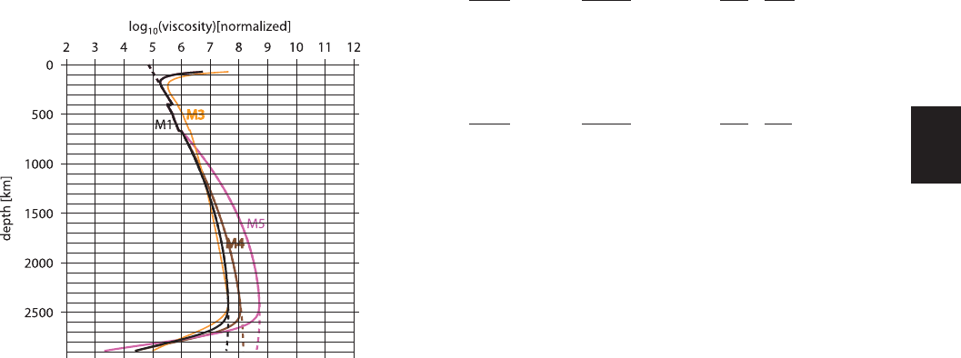
2.4 Normalized radial viscosity proﬁle—results

We can now express

η(z) = q

· η

· ˜η(z). (19)

is a constant scaling viscosity. ˜η(z) shown in Fig. 4 is the normal-

ized viscosity proﬁle proportional to F

(z) from eqs (7) and (11),

but adjusted by adding a constant to H in the lower mantle such that

the jump in H(z)/nR between upper and lower mantle is removed.

This adjustment is of no consequence to the results, and merely

serves to make the factors q

more easily interpretable. Without the

adjustment, ˜η(z) would increase by a factor ∼2000 from above to

below 660 km because of the different viscosity law assumed above

and below. This jump would be smaller for a lower value of g



, and

approximately removed for g



=8. Our results will show that such a

lower value of g



(corresponding to a less steep proﬁle in the lower

mantle) also increases the ﬁt to the geoid. Factors q

in individual

layers (lithosphere, upper mantle, one to two layers transition zone,

lower mantle) are treated as free parameters in the optimization dis-

cussed below. Figuratively speaking, the optimization consists of

shifting corresponding parts of the curves in Fig. 4 to the left or

right. ˜η(z) is only shown below depth 70 km, because the mecha-

nisms discussed here are not appropriate to model deformation of the

lithosphere, and lithospheric viscosity is treated as a free parameter.

It is shown for the same three cases as in Fig. 2. All proﬁles shown

Figure 4. Black and brown lines: non-optimized, normalized viscosity pro-

ﬁles for for the same cases as shown in Fig. 2. Additionally, the violet line

shows the proﬁle computed with g



= 20 instead, and the orange line shows

the proﬁle of Calderwood (1999). Dashed lines are adiabatic proﬁles, solid

lines are with thermal boundary layers. During the optimization, parts of

the proﬁles are shifted left or right relative to each other, yielding optimized

proﬁles as in Figs 9, 13, 14 and 15.

feature a characteristic hump in the lower mantle, like the proﬁles

derived by Ranalli (1995) for whole-mantle ﬂow. The curvature of

the hump depends on the curvature of the assumed melting curve.

For example, the proﬁle derived by Calderwood (1999) in a similar

manner is less curved in most of the lower mantle. The height of this

hump strongly depends on the value of g



and also depends on man-

tle potential surface temperature. Variations in the shape of the ˜η(z)

proﬁle in the lower mantle as a result of changing potential surface

temperature by ±100 K can be closely mimicked by appropriate

(small) changes in g



and are, therefore, not considered separately.

Whereas in the reference case, the viscosity increase from below

660 km to the maximum in the lower mantle is about a factor 40,

it is about a factor 100 for the brown line, although the only dif-

ference is a slightly smaller temperature increase towards the base

of the mantle, and it is even about a factor 500 for the violet line

with g



= 20. We, therefore, discuss the effect of g



on our model,

and which range of g



gives best results. Additionally, we discuss

the effect of d



and T

CMB

, corresponding to the thickness of the

basal mantle layer where viscosity is decreased, and to the total vis-

cosity decrease, and which combinations of T

CMB

and d



yield

optimal results. Steinberger & Holme (2006) extend this discussion

to include the effect of a basal layer with chemical variations.

2.5 Relation between seismic velocity variations

and temperature variations

If variations in seismic s wave speed are of thermal origin, they

relate to temperature variations through

δT = (δv

(z))/(∂ ln v

/∂T )

. (20)

δv

(z) are relative seismic wave speed variations, for which a

number of global tomography models exist. (∂ln v

/∂T )

is the

partial derivative of the logarithm of seismic s wave speed with re-

spect to temperature at constant pressure. Following Karato (1993),

it can be written as

−



∂ ln v

∂T



=−



∂ ln v

s,0

∂T



+ F(α) ·

−1

, (21)

whereby the ﬁrst term is the anharmonic part and the second one

the anelastic part. Q is the seismic Q-factor, and we set F(α) = 1.

With eq. (10) this becomes

−



∂ ln v

∂T



=−



∂ ln v

s,0

∂T



+ F(α) ·

−1

, (22)

in the lower mantle.

2.5.1 Anelastic part

We consider two Q proﬁles here: The ﬁrst one follows Anderson &

Hart (1978) except that a continuous instead of a stepwise proﬁle is

used. It is similar in shape to the logarithm of the non-dimensional

viscosity proﬁles ˜η(z) in Fig. 4, which makes intuitively sense, since

both anelasticity and viscosity are caused by similar mechanisms.

Because of this similarity, weuse the Anderson & Hart (1978) proﬁle

rather than a newer one. For the second proﬁle, we choose the shape

to exactly coincide with log(˜η(z)), hence we choose a, b and c such

that Q

(z) = a + bz + clog(˜η(z)) agrees with Anderson & Hart

(1978) at depths 250 km, 2400 km and the base of the mantle. Both

proﬁles for the anelastic part are shown in Fig. 5. In the reference

case, weusean anelastic part that is thearithmetic average for the two

cases described. Q is also expected to depend on temperature, hence



2006 The Authors, GJI, 167, 1461–1481

Journal compilation



2006 RAS

1468 B. Steinberger and A. R. Calderwood

Figure 5. Proﬁles of −(∂ ln v

/∂T )

, and contributing parts. Red line:

anharmonic part. Green lines: anelastic part. The dotted line is for the

Q-

proﬁle of Anderson & Hart (1978), the dashed line for Q

(z). Black line:

anharmonic plus anelastic part in the reference case (arithmetic average of

two green lines). Orange line: proﬁle derived by Calderwood (1999). The

blue line uses g = 30 for the anelastic part (eq. 22) instead. Brown line:

same case as in Figs 2 to 4. Other model assumptions are as in the reference

case.

a more accurate treatment should also consider lateral variations of

Q, for which models exist, at least in the upper mantle (Gung &

Romanowicz 2004).

2.5.2 Anharmonic part

For (∂ln v

s,0

/∂T )

we adopt the proﬁle given by Goes et al. (2004) in

the upper mantle. It is based on values for individual phases and the

mantle phase diagram of Ita & Stixrude (1992) for a pyrolite mantle,

using a geotherm similar to the reference case geotherm in Fig. 2.

In the lower mantle, (∂ln v

s,0

/∂T )

is recomputed to ensure con-

sistency with our proﬁle of α(z). We follow Duffy & Anderson

(1989) in assuming that radial derivatives of shear modulus μ for

different temperatures are related through

dμ

(

T (z) ±T (z)) =

dμ

(

T (z))(1 ±α(z)T (z)). (23)

This is based on the observation that in the PREM (Dziewonski &

Anderson 1981) lower mantle approximately

d ln



dμ



d ln ρ

≈−1, (24)

and the implicit assumption that this also holds along isobars.

μ(

T (z) ± T (z)) is determined by integrating eq. (23) along

adiabats, while computing temperature and thermal expansion co-

efﬁcients along the same adiabats. Starting point is

μ(T

lm,0

± T

) = μ(T

lm,0

) ±T

dμ

, (25)

at z =0. Based on parameters compiled by Cammarano et al. (2003)

and the pyrolite phase diagram of Ita & Stixrude (1992) it is es-

timated

dμ

= 27 MPa K

−1

for lower mantle mineralogy. T (z)

and α(z) are computed for the entire mantle with the lower man-

tle formulation described above. ‘Lower mantle potential surface

temperature’ T

lm,0

is found iteratively by matching the previously

determined lower mantle temperatures.

dμ

(T (z)) and μ(T

lm,0

) are

determined from the parameters of PREM layer 4, which comprises

most of the lower mantle. Thus

∂μ

∂T



≈

μ(

T (z) +T (z)) − μ(T (z) −T (z))

2T (z)

, (26)

is found, and with this (∂ ln v

s,0

/∂T )

can be computed (Fig. 5).

2.5.3 Sum of anharmonic and anelastic part

For the sum of anharmonic and anelastic part, agreement between

our reference case and Calderwood (1999) is good in the upper

mantle (Fig. 5), and would be even better if Q

(z) was used, but

our reference proﬁle is lower in the lower mantle: There, we choose

the factor g = 12 in the relation between activation enthalpy and

melting temperature. This value is much lower than previous es-

timates of g = 20–40 (Karato 1993) and thus leads to a smaller

anelastic contribution: The blue curve where g = 30 is used for

computation of the anelastic part (eq. 22) is higher in the lower man-

tle. The brown curve corresponds to somewhat lower temperatures

in the lowermost mantle (see Fig. 2) and is, therefore, also some-

what higher in the lowermost mantle. On the other hand, because

of the different way of computation, we compute a larger anhar-

monic part than Karato (1993) in the lower mantle. In our model,

the anharmonic part is larger below 660 km than above 660 km, be-

cause of larger values of

dμ

(Cammarano et al. 2003). Differences

for anharmonic and anelastic parts between our results and those

of Karato (1993) partly compensate each other, such that the sum

curve we obtain in our reference model is similar to that of Karato

(1993).

2.6 Relation between seismic velocity variations and

density variations

The scaling factor (∂ ln ρ/∂ ln v

)

is then obtained by dividing

thermal expansivity through −(∂ln v

/∂T )

(Fig. 6). In the refer-

ence case, it is similar to Calderwood (1999) in the upper man-

tle, but, corresponding to differences in Figs 3 and 5 somewhat

larger in the lower mantle. Again, the overall shape is similar to that

of Karato (1993). For the proﬁles derived here, the scaling factor

somewhat decreases with depth in the lower mantle, whereas the

Figure 6. Proﬁles of scaling factors (∂ ln ρ/∂ ln v

)

for the same cases

as in Figs 3 and 5. Additionally, the dotted blue line is with a

= 3.5 and

g = 30.



2006 The Authors, GJI, 167, 1461–1481

Journal compilation



2006 RAS

Large-scale mantle ﬂow and mineral physics 1469

proﬁle derived by Calderwood (1999) is almost constant over most

of the lower mantle, due to a smaller decrease of thermal expan-

sivity with depth. In the case with constant δ

(brown line), the

two effects of stronger decrease of thermal expansivity with depth

(Fig. 3) and less decrease of the −(∂ln v

/∂T )

proﬁle (Fig. 5)

combine to a much stronger decrease of scaling factor with depth.

A lower scaling factor in the lower mantle is obtained if either

alowerα

(black dashed line) or a larger g (blue lines) is as-

sumed. Changing potential surface temperature shifts the scaling

factor proﬁle (less than about ±10 per cent change for ±100 K po-

tential temperature change), and similar changes would also occur

if a different Q-factor proﬁle was used. Because we obtain simi-

lar changes also by changing F

, a

and/or g, changes in poten-

tial surface temperature and Q-factor proﬁle are not considered

separately.

In the reference model, the scaling factor is arbitrarily reduced,

compared Fig. 6, by a factor F

= 0.5 in the uppermost 220 km,

in order to account for the fact that density variations within the

lithosphere are probably only partly of thermal origin. Similarly,

other studies set density anomalies at lithospheric depths to zero

(Lithgow-Bertelloni & Silver 1998; Becker et al. 2003; Behn et al.

2004). However, we also consider the effect of varying F

on our

results and discuss which values give best results. In most cases,

and unless mentioned otherwise, we use tomography model smean

(Becker & Boschi 2002) for seismic velocity variations. Other to-

mography models are also considered.

3 OPTIMIZATION PROCEDURE

3.1 Mantle ﬂow computation

We can now combine a scaling factor proﬁle as derived in the pre-

vious section with an s-wave tomography model to obtain a density

model. With a viscosity proﬁle as described above, mantle ﬂow can

be computed. Equations of viscous ﬂow are solved with a spectral

method originally developed by Hager & O’Connell (1979, 1981):

Only radial viscosity variations are considered, thus the equations

decouple in the spherical harmonic domain and can be solved sep-

arately for each spherical harmonic. In the reference case, and if

not mentioned otherwise, spherical harmonic expansion is done up

to l

max

= 15, but cases with l

max

= 31 are considered as well. The

original method was modiﬁed to consider depth-dependent gravity

(from PREM), and to include the effects of compressibility (as de-

scribed in Steinberger 2000, following Panasyuk et al. 1996), and

of deﬂections δz of phase boundaries at depth 400 and 660 km in

thermal equilibrium. The latter effect was included as sheet mass

anomalies

δz · ρ =

ρ

· δρ , (27)

whereby δρ is the density anomaly as inferred from the tomogra-

phy model, at the depth of the phase transition. ρ

, γ

and α

are density, gravity and thermal expansivity at the phase bound-

ary. Values for ρ were given in the previous chapter. For ρ

the average value between above and below the phase boundary

(from the PREM model) is used, for α

, we use 2.079 ·10

−5

−1

660 km and 2.378 ·10

−5

−1

at 400 km—approximate average val-

ues between above and below the phase boundary from the reference

case in the previous chapter.

3.2 Variables in optimization

The optimization consists of ﬁnding the minimum of a misﬁt func-

tion in parameter space. Parameter space consists of the viscosity

factors q

, i =1 ...n

vis

in eq. (19). n

vis

is the number of layers where

viscosity is considered to vary independently. In most cases, we use

vis

= 4, in which case i = 1 corresponds to the lithosphere (0–

100 km), i = 2 the upper mantle (100–400 km), i = 3 the transition

zone (400–660 km) and i = 4 the lower mantle (below 660 km). In

some cases, the upper part of the transition zone (400–520 km) and

its lower part are considered separately. In this case, it is n

vis

=5, i =

3 corresponds to the upper part of the transition zone, i =4 its lower

part and i = 5 the lower mantle. Besides these parameters allowed

to vary within each optimization, variations are also considered for

a number of further parameters. These are kept constant within

each optimization, and the optimization is performed for several

sets of parameter values, and several 2-D grids in parameter space.

These further parameters include a

, b, g, g



, T

CMB

, d



and F

(see Table 1).

3.3 Haskell constraint

The Haskell constraint states that the logarithmic average of vis-

cosity, weighted with an appropriate sensitivity kernel equals about

Pa s. We express it in the form



CMB

120 km

log



η(r)

1Pas



· K (r) dr/



CMB

120 km

K (r) dr = 21, (28)

and use the sensitivity kernel for the Angerman River site given by

Mitrovica (1996) for K(r) (Fig. 7). If we choose η

such that, in

eq. (19) η

· ˜η(z) satisﬁes the Haskell constraint, we ﬁnd that η(z)

also does if 1.67 ·q

+1.33 ·q

≈0 in the case of one transition

zone layer, and 1.67 ·q

+ 0.67 ·q

+ 0.66 ·q

≈ 0 in the case

of two. We, therefore, choose the penalty function

= (1.67 · q

+ 1.33 ·q

)

, (29)

in the ﬁrst case, and a corresponding function in the second.

2500

2000

1500

1000

500

depth [km]

0 2 4 6 8 10 12

sensitivity kernel

Figure7. Kernel showing the sensitivity of post-glacial rebound to viscosity

at various depths. From Mitrovica (1996) for Angerman River.



2006 The Authors, GJI, 167, 1461–1481

Journal compilation



2006 RAS

1470 B. Steinberger and A. R. Calderwood

3.4 Heat ﬂux constraint

For each density ﬁeld and corresponding ﬂow ﬁeld, the advected

heat ﬂux is computed by integrating radial velocity v

times heat

anomaly δT ·C

·ρ =δ ln v

/(∂ ln v

/∂T )

·C

·ρ over spherical

surfaces at given depths:

(r) = C

· ρ/(∂ ln v

/∂T )



δ ln v

· v

dA. (30)

For this computation present-day surface plate motions (DeMets

et al. 1990) are used as boundary condition. This curve should ap-

proximately fall between theoretical steady-state proﬁles for an in-

ternally heated mantle and a basally heated mantle. Here we imple-

ment this constraint by penalizing if (r) >

or (r) <

(r).

For 

we use a constant value 33 TW representing our estimate

for the mantle heat ﬂux (Calderwood 1999), which is global heat

ﬂux minus heat produced in the crust. Pollack et al. (1993) compute

a global heat ﬂux 44 TW. By subtracting estimated heat production

in the continental crust from it, Schubert et al. (2001) estimate a

mantle heat ﬂux 37 TW. More recently, Hofmeister (2005) com-

puted a smaller global heat ﬂux 31 ± 1 TW, corresponding to only

about 24 TW mantle heat ﬂux. However, another recent analysis

(Wei & Sandwell 2006) yielded 42–44 TW. 

(r) has been modi-

ﬁed from the theoretical steady-state proﬁle for an internally heated

mantle with constant heat production rate per unit mass in order to

account for the fact that conduction is the dominant heat transport

mechanism close to the surface (see Fig. 8). We use the penalty

function



max



(r)−



, 0



+ max





(r)−(r)



, 0



2891 km

dr. (31)

Obviously, the assumption that heat ﬂuxat anydepth does not change

with time, which is implicitly made here, is not exactly satisﬁed for

the Earth. (r) is time variable and the present-day surface heat ﬂux

may be anomalously high or low. Hence we do not require P

= 0

exactly.

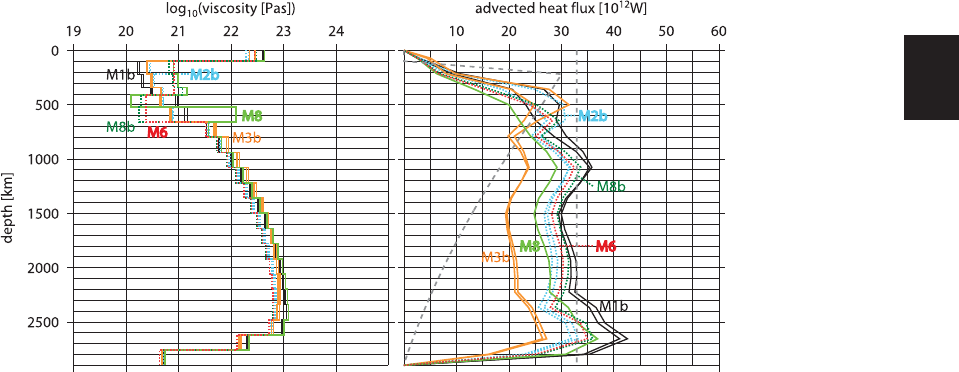
Figure 8. Optimized viscosity proﬁles (left) and advected heat ﬂux proﬁles (right), for cases where not all constraints are imposed. Orange lines: only heat

ﬂux and Haskell constraint. Violet lines: only geoid and Haskell constraint. Green lines: only geoid and heat ﬂux constraint. Red lines: viscosity proﬁle not

based on mineral physics but constant in lithosphere, upper mantle, transition zone and lower mantle. Continuous lines are with parameters as in the reference

case, dotted lines as in model 2. 

and 

(r) are shown as grey dashed lines. The heat ﬂux proﬁles should approximately lie in between.

3.5 Geoid constraint

For each density ﬁeld and corresponding ﬂow ﬁeld, the inferred

geoid is computed; ﬂow deforms boundaries, and both the density

anomalies that drive ﬂow and the deformed boundaries contribute

to the geoid. The inferred geoid is, therefore, quite sensitive to the

assumed viscosity structure. The ﬁt between computed and actual

geoid is expressed in terms of the penalty function

Var(Predicted–Observed)

Var(Observed)

. (32)

1 − P

is referred to as (geoid) variance reduction. For the geoid

computation, stress-free boundaries at the Earth’s surface and CMB

are assumed in the reference case; however, other boundary condi-

tions at the Earth’s surface are considered as well.

3.6 Misﬁt function

We optimize the model in parameter space by minimizing a misﬁt

function using a downhill simplex method (Press et al. 1986). This

method ﬁnds a local, not necessarily global minimum in parameter

space. In most cases, we will either minimize



= c

· P

+ c

· P

+ P

, (33)

(misﬁt criterion 1) or require the Haskell constraint to be ﬁt exactly,

and minimize



= c

· P

+ P

, (34)

under the additional constraint P

= 0 (misﬁt criterion 2, corre-

sponding to criterion 1 with c

−→ ∞ ). Cases indicated with a

star in Table 2 use criterion 2 (except for M17, M17b in Section 4.9

which use a modiﬁed criterion), all others (including those in Figs 11

and 12, but except for cases M19 and M19b in Table 1 and Sec-

tion 4.2) use criterion 1. In most cases, we will use c

= 1, c

= 4. We ﬁnd that results remain very similar with both criteria,

and hence do not strongly depend on c

, as the Haskell constraint

is always ﬁt very well. The value for c

is discussed in the next

section.



2006 The Authors, GJI, 167, 1461–1481

Journal compilation



2006 RAS

Large-scale mantle ﬂow and mineral physics 1471

Table 2. List of numerical models. The ‘comments’ column indicates differences to the reference model, except for ‘b’ models, where it

indicates the difference to models without ‘b’. VR is geoid variance reduction, P

heat ﬂow misﬁt (eq. 31). Numbers in brackets indicate

either results with expansion up to l

max

= 31 (M1–M3b), or with model 2 parameters (M7–21). Stars indicate cases where an exact ﬁt

to the Haskell constraint has been prescribed. UM-upper mantle, TZ-transition zone, LM-lower Mantle.

Model # comment VR [per cent] P

∗

Reference case 75.9 (74.7) 0.0165 (0.0133)

M1b

∗

Lowest viscosity in asthenosphere 71.6 (70.5) 0.0125 (0.0090)

∗

= 3.5, g = 30 79.7 (78.6) 0.0133 (0.0099)

M2b Lowest viscosity in asthenosphere 76.0 (75.4) 0.0109 (0.0078)

∗

Based on Calderwood (1999) 79.5 (78.5) 0.0122 (0.0093)

M3b Lowest viscosity in asthenosphere 75.3 (74.6) 0.0105 (0.0076)

∗

= 5.5 constant 65.7 0.0044

M4b

∗

Lowest viscosity in transition zone 52.8 0.0140

∗



= 20 −15.5 0.0356

∗

η = const in UM, TZ; model 2 parameters 79.6 0.0138

M7 (M7b) η = const in UM, TZ, LM 81.2 (80.8) 0.0163 (0.0143)

∗

(M8b

∗

) Independent η in upper, lower TZ 80.0 (79.7) 0.0164 (0.0131)

∗

(M9b

∗

) Tomography model S20RTS 74.2 (76.1) 0.0129 (0.0114)

M10

∗

(M10b

∗

) Tomography model SB4L18 47.9 (64.6) 0.0175 (0.0052)

M11

∗

(M11b

∗

) Tomography model Grand (2002) 67.7 (69.0) 0.0250 (0.0296)

M12

∗

(M12b

∗

) Tomography model SAW24B16 64.7 (74.3) 0.0187 (0.0154)

M13

∗

(M13b

∗

) Tomography model S12WM13 44.3 (56.0) 0.0188 (0.0086)

M14

∗

(M14b

∗

) Tomography model S362D1 55.9 (69.3) 0.0116 (0.0066)

M15

∗

(M15b

∗

) Fixed surface 38.4 (45.8) 0.0138 (0.0194)

M16 (M16b) Plates moving half free speed 11.2 (19.1) 0.0082 (0.0052)

M17

∗

(M17b

∗

) Plates free speed, tractions at surface, v

rms

penalty 24.1 (31.0) 0.0068 (0.0130)

M18

∗

(M18b) Prescribed plate motions 13.9 (14.8) 0.0029 (0.0034)

M19 (M19b) Only heat ﬂux and Haskell constraint −3140.3 (−1923.6) 0.0000 (0.0001)

M20

∗

(M20b

∗

) Only geoid and Haskell constraint 78.0 (79.7) 0.1133 (0.0134)

M21 (M21b) Only geoid and heat ﬂux constraint 78.0 (79.5) 0.0173 (0.0138)

4 RESULTS

4.1 Overview

We ﬁrst show optimized viscosity and heat ﬂux proﬁles (Fig. 8), as

well as variance reduction and heat ﬂow misﬁt P

for cases where

the constraints are not all imposed simultaneously (M7, 7b, 19–21b

in Table 2). This includes one case with constant viscosities in dif-

ferent mantle layers instead of proﬁles based on mineral physics.

We then go on to imposing all constraints simultaneously and show

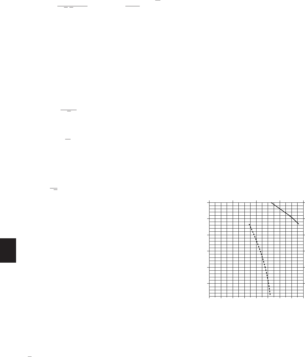
Figure 9. Optimized viscosity proﬁles (left) and advected heat ﬂux proﬁles (right). Colour and type of lines correspond to Figs 4 and 6. 

and 

(r) are

shown as grey dashed lines. Per diagram there are two black, orange and blue lines: one, with higher heat ﬂux values in the upper mantle, was computed with

max

= 31, the other with l

max

= 15.

results for our reference model (M1; Figs 9 and 10), further ‘pre-

ferred’ models (M2 with a

=3.5 and g =30, and M3 with proﬁles

from Calderwood (1999)) and further models (M4, M4b and M5)

with stronger depth dependence of either lower mantle viscosity

or thermal expansivity (Fig. 9). We then systematically vary pa-

rameters a

, g, g



, n = g/g



, T

CMB

, d



and F

within bounds as

listed in Table 1, and present contour plots of optimized variance

reduction (Fig. 11) and heat ﬂow misﬁt P

(Fig. 12) as a function

of two of these parameters. Subsequently, we consider results with



2006 The Authors, GJI, 167, 1461–1481

Journal compilation



2006 RAS

1472 B. Steinberger and A. R. Calderwood

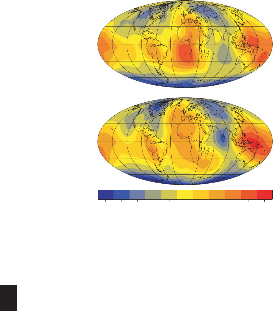
observed

predicted

-100 -80 -60 -40 -20 0 20 40 60 80 100

geoid in m

Figure 10. Above: geoid computed for the reference case. below: observed geoid.

the further constraint that viscosity is lowest in the asthenosphere

(M1b, M2b, M3b), with constant viscosity in the upper mantle and

transition zone (M6) viscosity in the upper and lower part of the

transition zone varying independently (M8, 8b) (all in Fig. 13), dif-

ferent tomography models (M9–14b; Fig. 14), and different surface

boundary conditions (M15–18b; Fig. 15).

4.2 Cases where not all constraints are imposed

simultaneously

Discussing model cases where not all constraints have been im-

posed helps clarifying which features of the results are due to which

constraints. Since the geoid ﬁt is only affected by relative viscosity

variations, we need at least one additional constraint for the abso-

lute viscosity level—either the Haskell or the heat ﬂux constraint.

If we impose geoid and Haskell constraint (use misﬁt criterion 2

with c

= 0) we obtain a geoid variance reduction of 78 per cent or

80 per cent with other assumptions as in the reference case (M20)

or in case M2 (M20b). Resulting viscosity structure (violet lines in

Fig. 8, left-hand side panel) is very similar in both cases. For M20,

the computed heat ﬂux is too large in the lower mantle (continuous

violet line in Fig. 8, right-hand side panel), whereas for M20b (dot-

ted violet line) it matches the observation-based estimate of mantle

heat ﬂux quite well, even without imposing any heat ﬂux constraint.

If we impose instead geoid and heat ﬂux constraint (use misﬁt cri-

terion 1 with c

=0 and c

=4), we obtain heat ﬂux proﬁles (green

lines in Fig. 8, right-hand side panel) similar to M20b. The opti-

mized viscosity structure in case M21b (dotted green line in Fig. 8,

left-hand side panel) remains very similar to case M20b, that is, the

Haskell constraint is matched well in M21b even without impos-

ing it. In case M21 (continuous green line), viscosity is somewhat

higher than in case M20 by approximately a factor 1.6 throughout

the mantle. Geoid variance reduction (78 per cent in M21 and 79

per cent in M21b) remains similar to cases M20 and M20b, hence

with this relative weighting of geoid and heat ﬂux constraint (c

4) the latter is not overly constraining.

We ﬁnd that both Haskell and heat ﬂux constraint can be simul-

taneously ﬁt almost perfectly (M19 and M19b); therefore, there is

no beneﬁt in looking at cases with only one of them imposed. Re-

sulting viscosity and heat ﬂux proﬁles if we impose Haskell and

heat ﬂux constraint (i.e. minimize 

in eq. (33) with c

= 1,

=4, and without the term P

) are shown as continuous (M19) and

dotted (M19b) orange lines in Fig. 8. However, there is a huge misﬁt

between predicted and observed geoid. Thus, the geoid constraint

is the most essential one.

Finally, with constant viscosities in upper mantle, transition zone

and lower mantle we are able to obtain geoid variance reduc-

tion 81 per cent and reasonable heat ﬂux proﬁles (cases M7 and

M7b), with lower mantle viscosity of about 3 · 10

Pa s. This is

similar to results obtained in previous work. The main objective

of this paper is to ﬁnd out whether we can replace the assump-

tion of layers with constant viscosities (in particular in the lower

mantle) with viscosity proﬁles based on mineral physics without

substantially degrading the ﬁt to the geoid, heat ﬂux and Haskell

constraints.



2006 The Authors, GJI, 167, 1461–1481

Journal compilation



2006 RAS

Large-scale mantle ﬂow and mineral physics 1473

Figure 11. Geoid variance reduction as a function of a

and g (but g



=12 constant) (top left), of g



and n =g/g



(top right), of g = g



and T

CMB

(centre right),

of d



and T

CMB

(centre left), and of d



and F

(bottom left); other parameters as in the reference case. These are cross-sections through a 5-D parameter

space intersecting along the grey lines S1, S2, S3 and S4. For each point, the model has been optimized by minimizing the misﬁt function P

+ 4P

+ P

a 4-D parameter space. The thick black line divides regions where the lowest viscosity occurs in the transition zone from where it occurs in the asthenosphere

(indicated by the letter ‘a’). Location of models M1, M2 and M5 is also indicated.

4.3 Reference case

Fig. 10 compares the predicted geoid with the observed one in the

reference case (M1). The variance reduction is 76 per cent. This is

slightly less than in cases M20 and M21 above—as more constraints

are imposed simultaneously, the ﬁt to the geoid is somewhat reduced.

The optimized viscosity model and corresponding advected heat

ﬂux proﬁles for cases given in Figs 4 and 6 are shown in Fig. 9; for

the reference case (black lines), the difference between the lowest

viscosity (in the transition zone) and the highest viscosity at the base

of the mantle is about a factor 700. With the relative weighting of

geoid and heat ﬂux constraint c

= 4 variance reduction decreases

by only a few per cent compared to the case without any heat ﬂux

constraint. At the same time the heat ﬂux constraint is probably

ﬁt well enough considering possible time variations in heat ﬂux

mentioned above. We will hence maintain this relative weighting in

what follows.

4.4 Dependence on thermal expansivity and relation

between s wave speed and temperature

We can achieve an even higher variance reduction with a somewhat

higher α and larger g in eq. (22) while keeping g



=12 in the viscosity

law eq. (11), resulting in higher values of −(∂ln v

/∂T )

and lower

values of (∂ ln ρ/∂ ln v

)

. For example, the model with a

= 3.5

and g = 30 (M2; blue dotted lines) gives a variance reduction of

80 per cent. Also, the heat ﬂux proﬁle now ﬁts even better, as it

stays below 34 TW throughout the mantle. We saw above for cases

M20b and M21b that with these parameters a good ﬁt to the heat

ﬂux or Haskell constraint is obtained even without applying those

constraints. Hence it is not surprising that results stay very similar

if, in case M2, we apply these constraints simultaneously.

Also, if both proﬁles for thermal expansivity and −(∂ ln v

/∂T )

are adopted from Calderwood (1999), a variance reduction of

80 per cent is achieved along with a suitable heat ﬂux proﬁle



2006 The Authors, GJI, 167, 1461–1481

Journal compilation



2006 RAS

1474 B. Steinberger and A. R. Calderwood

Figure 12. Misﬁt P

, as deﬁned in eq. (31), of the heat ﬂux proﬁle for the same cross-sections and models as in Fig. 11, where further explanations are given.

(M3; orange lines). However, heat ﬂux in the uppermost few 100 km

below the lithosphere is under-predicted in all three models dis-

cussed so far—and this is in fact a general problem with all models

that give otherwise a good ﬁt. Likely explanations for this misﬁt

are discussed in the last section. This misﬁt is somewhat less with

max

= 31. In this case geoid variance reduction is slightly reduced

to 75, 79 and 78 per cent, respectively, for the three cases M1, M2

and M3 considered thus far.

The dependence of variance reduction and misﬁt function on g

used in the velocity-temperature relation eq. (22) and a

, but keeping



= 12 in the viscosity law eq. (11) is further illustrated in the top

left panels of Figs 11 and 12: If a

and g are both increased relative to

the reference case g =12, both geoid variance reduction and the heat

ﬂux proﬁle are somewhat improved. For g =12 the highest variance

reduction is obtained with somewhat smaller a

≈ 3 whereas for

g =42 itis obtained with somewhatlarger a

≈4; both combinations

yield values of (∂ ln ρ/∂ ln v

)

≈ 0.3 in the lower mantle, which

appears to work best for achieving a good ﬁt to the geoid.

The better ﬁt of the heat ﬂux proﬁle for larger g is a result of

the higher values of −(∂ ln v

/∂T )

in the lower mantle, resulting

in lower temperature anomalies inferred from seismic tomography,

thus lower inferred heat ﬂux. Probably the improved variance reduc-

tion for larger g is due to the same reason; once the heat ﬂux con-

straint becomes less difﬁcult to satisfy, the optimization can rather

focus on optimizing the ﬁt to the geoid.

In the case of a stronger decrease of α with depth (no depth

dependence of δ

, that is, b =0; M4; brown lines in Fig. 9) variance

reduction is reduced to 66 per cent. Both the resulting optimum

viscosity structure with a rather high transition zone viscosity and

heat ﬂux proﬁle look somewhat unrealistic. If, in this case, the lowest

viscosity is restricted to occur in the transition zone, proﬁles look

more realistic, but variance reduction in this case (M4b) is further

reduced to 52 per cent. Thus, the smaller decrease of α with depth in

the reference case appears more appropriate to achieve good results.

This is probably partly due to the fact that a constant δ

leads to less

temperature increase with depth, hence a steeper viscosity proﬁle.



2006 The Authors, GJI, 167, 1461–1481

Journal compilation



2006 RAS

Large-scale mantle ﬂow and mineral physics 1475

4.5 Dependence on lower mantle viscosity

A steeper viscosity proﬁle is also obtained with a larger value of



. With g



= 20 (M5; violet lines in Fig. 9), we obtained a vari-

ance reduction of only −15 per cent and the heat ﬂux proﬁle also

looks unrealistic. The dependence of variance reduction and heat

ﬂux misﬁt on the steepness of the viscosity proﬁle is further illus-

trated in the centre right panels of Figs 11 and 12: The viscosity

increase through the lower mantle becomes larger with increasing



, the viscosity drop at the base of the mantle becomes larger with

increasing T

CMB

. An increase of either of them relative to the ref-

erence case leads to substantial deterioration of both the predicted

geoid and heat ﬂux proﬁle, but decrease does not yield substantial

improvement. In fact, low values of g tend to also give a larger misﬁt

of the heat ﬂow proﬁle; this arises, as the viscosity hump in the lower

mantle is then less high, and thus the heat ﬂux predicted tends to be

too high in part of the lower mantle.

The top right panels of Figs 11 and 12 show that the deteriorating

ﬁt with increasing g and g



in the centre right panels is in fact due to

the viscosity proﬁle; if we leave g



constant in the viscosity relation

eq. (11) but increase g =g



n in eq. (22) through increasing n, the ﬁt

rather tends to improve—for reasons already discussed for the top

left panels.

There is also a trade-off between the assumed temperature at

the base of the mantle and the thickness of the thermal boundary

layer d



at its base, as shown in the centre left panels of Figs 11

and 12: For d



≈ 350 km, the highest geoid variance reduction

is obtained with T

CMB

≈ 3000 K, for d



≈ 200 km with T

CMB

≈

3500 K (reference case), andfor d



≈125 km with T

CMB

≈4000 K.

The smallest heat ﬂow misﬁt tends to occur with somewhat smaller

thermal boundary layer thicknesses and/or CMB temperatures, as

this gives smaller predicted heat ﬂux in the lowermost mantle, which

is too high in the reference model.

4.6 Dependence on upper mantle velocity

to density scaling

In the reference model, the scaling factor is arbitrarily reduced by

a factor F

= 0.5 in the uppermost 220 km, in order to account

Figure 13. Optimized viscosity proﬁles (left) and heat ﬂux proﬁles (right). Black, orange and dotted blue lines (two per diagram) correspond to Figs 9, but

with the restriction that lowest viscosities are to occur in the asthenosphere. Light green and dark green dotted lines are for the same models as black and blue

dotted lines, but with viscosities in the upper and lower transition zone independently varying. 

and 

(r) are shown as grey dashed lines. Red dotted lines

are for the same case as blue dotted, but with constant viscosities 100–410 and 410–660 km.

for the fact that density variations within the lithosphere are prob-

ably only partly of thermal origin. The bottom left panel of Fig. 11

shows that this is in fact an appropriate choice; the highest variance

reduction occurs for intermediate values of F

around 0.5, but the

ﬁt to the geoid does not strongly depend on F

. On the other hand,

the bottom left panel of Fig. 12 shows that a better ﬁt to the heat

ﬂow proﬁle is obtained with larger F

, because this increases the

computed heat ﬂow below the lithosphere, thus reducing the misﬁt

there, particularly in cases where the lowest viscosity occurs in the

asthenosphere.

4.7 Dependence on upper mantle and transition

zone viscosity

The resulting optimized viscosity structure remains very similar

in all three cases included in Fig. 9 that give good results—the

reference case, model 2 and the case with proﬁles from Calderwood

(1999); it shows a pronounced viscosity decrease in the transition

zone—about one order of magnitude relative to above or below.

In order to assess whether the result that the lowest viscosity in

our reference model occurs in the transition zone is of signiﬁcance,

we also include an optimization restricted to models with transition

zone viscosities higher than in the upper mantle. The variance re-

duction is then slightly reduced to 72 per cent (71 per cent) with

reference case parameters (M1b), 76 per cent (75 per cent) with

model 2 parameters (M2b), and 75 per cent (75 per cent) with the

proﬁles from Calderwood (1999) (M3b) (numbers in brackets with

max

= 31). The heat ﬂux proﬁle remains very similar, and the vis-

cosity maximum in the lower mantle remains similar at about, or

slightly below 10

Pa s for all three models (Fig. 13). We ﬁnd a

general tendency that models with lowest viscosity in the transition

zone tend to yield somewhat higher variance reduction than models

with the lowest viscosity in the asthenosphere (Fig. 11). It is hard

to judge whether this slightly reduced variance reduction warrants

attaching signiﬁcance to the result that the lowest viscosity occurs

in the transition zone. The best ﬁt of the heat ﬂux proﬁle is obtained

for cases where the lowest viscosity occurs in the asthenosphere,

since this allows for a higher heat ﬂux in the uppermost few 100 km

below the lithosphere, thus reducing the misﬁt there (Fig. 12).



2006 The Authors, GJI, 167, 1461–1481

Journal compilation



2006 RAS

1476 B. Steinberger and A. R. Calderwood

Results stay very similar, if the viscosity is kept constant in the

upper mantle, and constant in the transition zone (Fig. 13, red dotted

lines). This conﬁrms that results—as stated in Section 2.2.2—do

not strongly depend on the activation enthalpy proﬁle in the upper

mantle. Furthermore, we consider the case that viscosity in the upper

and lower part of the transition zone, that is, above/below 520 km,

varies independently; in the reference case, this leads to an increase

in variance reduction to 80 per cent, with a rather strong viscosity

contrast between the upper and lower part of the transition zone. In

model 2, variance reduction remains 80 per cent, and the optimized

viscosity structure remains very similar. We, therefore, regard the

constraints of our method as insufﬁcient to resolve details of the

viscosity structure such as the difference between the upper and

lower part of the transition zone. We also computed results without

consideration of phase boundaries, for an incompressible mantle,

and for the two different Q proﬁles; in all cases results stay very

similar, and are therefore not shown.

4.8 Dependence on tomography model

Fig. 14 shows results for different tomography models with model

2 parameters. In most cases, the smallest misﬁt occurs with the

lowest viscosity in the transition zone, only for SB4L18 (M10b) the

smallest misﬁt occurs with the lowest viscosity in the asthenosphere.

With reference case parameters, this happens with SB4L18 (M10),

Grand’s model (M11), SAW24B16 (M12) and S362D1 (M14). The

resulting maximum viscosity in the lower mantle is very similar for

all models—around, or slightly below 10

Pa s. There are quite

large differences between the heat ﬂux proﬁles for various models.

Largely these are due to the differences in rms amplitudes versus

depth among the tomography models. For example, Grand’s model

(blue lines) has higher rms amplitudes than S20RTS (red line) in

the lowermost mantle, but lower amplitudes between ≈1500 and

300 km depth. The model smean (black) is an average of Grand’s

model (blue), S20RTS (red) and SB4L18 (green) and gives a heat

ﬂux proﬁle that is approximately constant through much of the man-

tle. Geoid variance reductions and heat ﬂow misﬁt P

of optimized

models are listed in Table 2. There is a general tendency for better

Figure 14. Optimized viscosity proﬁles (left) and heat ﬂux proﬁles (right) for different tomography models. Other assumptions are as in model 2. Black: smean

(Becker & Boschi 2002)—identical to the blue dotted line in Fig. 9; red: S20RTS (Ritsema & van Heijst 2000); green: SB4L18 (Masters et al. 2000); blue:

model by Grand (2002); violet: SAW24B16 (M´egnin & Romanowicz 2000); orange: S12WM13 (Su et al. 1994); brown: S362D1 (Gu et al. 2001). 

and



(r) are shown as grey dashed lines.

ﬁt with model 2 parameters, which gives smaller density anomalies.

In particular, the difference is pronounced for those models with

comparatively large amplitudes away from the boundaries, that is,

where geoid kernels are larger—such as SB4L18. Such models give

generally lower variance reduction, as they would presumably re-

quire even lower conversion factors from seismic velocity to density

anomalies in order to yield a good ﬁt. Models with lower amplitudes

(S20RTS, Grand) tend to give better ﬁt and the difference between

the ﬁts with reference case parameters and model 2 parameters is

smaller. However, with no individual tomography model we were

able to exceed the variance reductions obtained with the average

model smean.

4.9 Dependence on upper boundary condition

Upper boundary condition for the computation of the geoid in the

models discussed thus far was a free surface. Since this is not entirely

appropriate for a surface broken into plates not well characterized

by viscous rheology, we show in Fig. 15 results for different sur-

face boundary conditions. For ﬁxed surface, variance reduction of

the optimized models with reference case parameters (M15, grey

lines) is 38 per cent, with model 2 parameters (M15b, black lines)

it is 46 per cent. With plates moving freely according to the forces

acting on them due to mantle ﬂow, with tractions applied at the

base of the plates at depth 100 km (see Steinberger et al. 2001,

for a detailed description of the methodology) we obtain a negative

variance reduction—also plates are moving too fast compared to

observations. Thus, we go on to a case with plates moving at half

the speed of free plate motions. In this case (M16, green lines with

reference case parameters; M16b, red lines with model 2 parame-

ters), calculated rms plate motions v

rms,c

are 5.2 cm yr

−1

(M16) and

5.3 cm yr

−1

(M16b), similar to the observed v

rms,o

= 4.4 cm yr

−1

For the difference between predicted and observed plate motions,

rms values are 3.8 cm yr

−1

in both cases, corresponding to plate

motion variance reductions of 25 per cent (M16) and 23 per cent

(M16b). Geoid variance reduction remains low at 11 per cent

(M16) and 19 per cent (M16b). A similar geoid variance reduc-

tion is obtained with prescribed plate motions (13.9 per cent and



2006 The Authors, GJI, 167, 1461–1481

Journal compilation



2006 RAS

Large-scale mantle ﬂow and mineral physics 1477

Figure 15. Optimized viscosity proﬁles (left) and heat ﬂux proﬁles (right) for different surface boundary conditions. Fixed surface for reference case (grey)

and model 2 (black); plates moving at half the speed of free plate motions, for tractions applied at the base of the lithosphere at 100 km depth for refere

nce

case (green) and model 2 (red); free plate motions for tractions applied at the surface, with additional penalty added to misﬁt function if computed rms surface

plate motions differs from observed one for reference case (blue) and model 2 (orange). 

and 

(r) are shown as grey dashed lines.

14.8 per cent in cases M18 and M18b). This rather poor model per-

formance arises, because plate-like surface motions do not naturally

arise with a viscous rheology, and if they are artiﬁcially imposed,

artefacts occur in the computed geoid, which degrade the ﬁt. The

optimized models in this case show rather low viscosities in the up-

per 100 km as in this way artefacts are kept small. Using stresses

at depth 100 km for computing plate motions, if the model does

not contain a high-viscosity lithosphere above, also appears inap-

propriate. We, therefore, go on to a case where we apply stresses

at the surface. For this case, optimized models have very high vis-

cosity in the uppermost 100 km and very slow plate motion; result-

ing sublithospheric viscosity and heat ﬂux proﬁles are very simi-

lar to the ﬁxed surface case shown. In the last case we, therefore,

add

= (1 − v

rms,c

rms,o

)

, (35)

to the misﬁt function 

in eq. (34), that is, penalizing if calculated

and observed rms plate motions differ. Then we obtain for reference

case parameters (M17, blue lines) a geoid variance reduction of 24

per cent, v

rms,c

is 4.0 cm yr

−1

and plate motion (i.e. surface velocity)

variance reduction 56 per cent. For model 2 parameters (M17b,

orange lines) corresponding numbers are 31 per cent, 3.8 cm yr

−1

and 58 per cent. Viscosities in the upper 100 km are a few times

Pa s—as with a free surface in the three cases discussed that

give a high geoid variance reduction—the reference case M1, model

2 (M2) and the case M3 with proﬁles from Calderwood (1999). For

these three cases, v

rms,c

is 3.3, 5.0 and 4.6 cm yr

−1

, surface velocity

variance reduction is 28, −5 and 4 per cent. Thus, these models with

free surface give approximately correct rms surface velocities even

though these are not used as constraints; lithospheric viscosities (to

be interpreted as effective viscosity along plate boundaries) required

to obtain a good ﬁt to the geoid are in the same range as those

required to obtain appropriate plate speeds. These results do not

change substantially if we penalize a misﬁt of rms plate motions

as described. The smaller surface velocity variance reduction in

models M1, M2 and M3 can be attributed to the fact that here surface

velocities are not plate-like.

5 DISCUSSION AND CONCLUSIONS

5.1 Resulting viscosity proﬁles

We have derived here mantle viscosity proﬁles with a combina-

tion of mineral physics and mantle dynamics. They feature a strong

viscosity increase with depth in the lower mantle up to about

Pa s or slightly less above the D



layer, several hundred times

more than the viscosity low in the upper mantle. This is a larger vis-

cosity contrast than previously inferred from the geoid constraint

in global geodynamics (e.g. Thoraval & Richards 1997). We obtain

this larger contrast because our resulting viscosity models have a

characteristic hump in the lower mantle; preferred models feature a

viscosity increase of about a factor 30 from below the 660 km dis-

continuity to the viscosity high in the lower mantle, and a viscosity

decrease of somewhat more than a factor 100 from the viscosity high

to the CMB. Models with much larger viscosity increase through the

lower mantle tend to give a much higher misﬁt and are, therefore,

considered less likely. Models with much larger viscosity decrease

in the lowermost mantle also tend to give much higher misﬁt, unless

the thermal boundary layer at the base of the mantle is much thinner.

Because the highest viscosities are restricted to the deep mantle, they

are also compatible with results from post-glacial rebound, which is

rather insensitive to viscosities at that depth.

The combination of mineral physics, geoid and heat ﬂux con-

straints applied here was motivated by the fact that the geoid alone

does not place strong constraints on mantle viscosity structure

(Thoraval & Richards 1997). However, we found that our model

still leaves considerable uncertainties; for example, we cannot reli-

ably distinguish whether the lowest viscosities occur in the astheno-

sphere or in the transition zone; generally, a somewhat better model

ﬁt occurs with lowest viscosities in the transition zone. This was

e.g. also found by Marquart (2006). A possible explanation could

be the presence of water in the transition zone (Smyth et al. 2004;

Kavner 2003). Such a viscosity low serves to somewhat decouple

ﬂow in the upper and lower mantle, which appears to improve the

ﬁt to the geoid. However, this can also be achieved by narrow lay-

ers of low viscosity (Panasyuk & Hager 2000; Mitrovica & Forte

2004).



2006 The Authors, GJI, 167, 1461–1481

Journal compilation



2006 RAS

1478 B. Steinberger and A. R. Calderwood

If we require the lowest viscosities to occur in the asthenosphere,

then best-ﬁt viscosity models look similar to the proﬁle obtained

by Mitrovica & Forte (2004) without mineral physics constraints. A

difference is the narrow layer of low viscosity above depth 670 km

which occurs in the model of Mitrovica & Forte (2004), and which

is not possible with our parametrization.

With alternative surface boundary conditions (ﬁxed or plate-like)

the best-ﬁt models have the lowest viscosity in the asthenosphere.

Any indication of a viscosity low in the transition zone could, there-

fore, merely reﬂect the inappropriate surface boundary condition

and neglect of lateral variations in rheology. However, this will need

to be addressed by future studies.

5.2 Fit to the geoid

Our best-ﬁt models with viscosity and scaling factor proﬁles based

on mineral physics give a geoid variance reduction of about 80 per

cent. This is similar to values achieved by previous authors, how-

ever, we were able to obtain this result in a parameter space that is

rather small, as we use mineral physics to pre-constrain the viscosity

structure and conversion factor from seismic velocities to densities.

A variance reduction close to 80 per cent could be achieved for a

range of modelling parameters, but not be substantially exceeded.

With constant viscosities in upper mantle, transition zone and

lower mantle, we obtain a slightly higher geoid variance reduction

(81 per cent). However, we want to replace ad hoc assumptions

(such as constant viscosities) by models based on mineral physics.

We regard the outcome that this only leads to a slightly worse ﬁt to

the geoid, while at the same time a realistic heat ﬂux proﬁle (see

discussion below) is maintained as quite satisfactory.

A geoid variance reduction of slightly more than 80 per cent ap-

pears to be the approximate limit that can be achieved with the inter-

pretation of seismic wave speed anomalies purelyin terms of thermal

anomalies, and without consideration of lateral viscosity variations.

Like Thoraval & Richards (1997), we obtained the best result with

a free-slip surface boundary condition—probably, because this is

the boundary condition that is consistent with the purely viscous

rheology without lateral variations that we also use to model the

lithosphere; plate-like surface velocities without lateral variations

in rheology in the lithosphere lead to artefacts in the computed

geoid.

The good ﬁt to the geoid obtained is indicative that at depths

where the geoid kernels (showing the sensitivity of the geoid to den-

sity variations) are comparatively large—away from the surface and

CMB—seismic anomalies are primarily due to temperature anoma-

lies. This leaves the regions close to the surface and close to the

CMB as potential regions for large chemical variations: Our ﬁnding

that the ﬁt to the geoid is somewhat improved, if the conversion fac-

tor from seismic velocities to densities is reduced by about a factor

0.5 in the upper 220 km, may be additional evidence that part of

the density anomalies in the uppermost mantle are due to compo-

sitional, rather than thermal anomalies. A more detailed treatment

of the shallowest mantle would need to consider the non-linear de-

pendence of seismic velocity on temperature anomalies; the same

temperature variation causes larger s wave speed variation at lower

temperature than at higher temperature (Cammarano et al. 2003).

On the other hand, surface velocity variance reduction obtained

is highest with plate-like surface motions. This points towards the

need of combining mineral physics constraints with geodynamic

models that include lateral variations in rheology—particularly in

the uppermost mantle (

Cadek & Fleitout 2003).

5.3 Heat ﬂux

In addition to a high geoid variance reduction, our best-ﬁt models

also give heat ﬂux proﬁles that are compatible with the observation-

based mantle heat ﬂux. Heat ﬂux proﬁles are quite variable for

different density models—based on different mantle tomography

models—used, but our best-ﬁt models have a roughly constant heat

ﬂux through much of the mantle, corresponding to a mantle largely

heated from below. The rather small fraction of plume heat ﬂux

compared to total surface heat ﬂux has frequently been taken as

evidence for a largely internally heated mantle. However, much

higher values of plume ﬂux have recently been inferred with the

help of seismic tomography (Nolet et al. 2005). Experimental re-

sults (Jellinek et al. 2003) have shown that a signiﬁcant fraction of

core heat ﬂux can be drawn into large-scale upwellings and is thus

not observed at hotspots. A large part of core heat ﬂux may be due

to warming of slabs settling on the CMB (Yoshida & Ogawa 2005;

Mittelstaedt & Tackley 2006). If seismic velocity anomalies are

due to temperature anomalies, the skewness of s-wave tomography

models suggests signiﬁcant basal heating (Yanagisawa & Hamano

1999).

Predicted heat ﬂux is generally too low in the uppermost few

hundred km. This may be due to a number of reasons:

(i) The scaling factor in the uppermost 220 km has been arbi-

trarily reduced by a factor F

= 0.5; the misﬁt becomes smaller for

larger F

(Fig. 12).

(ii) Heat ﬂow in the lithosphere is dominated by diffusion, which

is not included in our computation, and in many places the litho-

sphere is probably considerably thicker than the 100 km assumed

here.

(iii) Probably a substantial fraction of heat ﬂux occurs through

subduction of lithospheric slabs, and those are not fully resolved

in our model (expansion up to degree 31), especially in the upper

mantle. Heat ﬂow misﬁt P

for expansion up to degree l

max

= 31 is

less than for l

max

= 15. The largest differences occur in the upper

part of the mantle. Most density models used here to drive mantle

ﬂow are expanded to degree 31 or less, and we expect that P

would

be further reduced if density and ﬂow models were expanded to

larger l

max

(iv) Further heat ﬂux at shorter wavelength may occur through

small-scale convection, primarily in the regions with lowest vis-

cosity. Since the remaining heat ﬂux misﬁt is primarily in the depth

region 100–400 km, small-scale convection could explain part of the

misﬁt, especially if the lowest viscosities also occur in that depth

range.

In our reference model, heat ﬂux in the lower mantle tends to be

somewhat too high. Better results are obtained in model 2, where

temperature anomalies are less. While the amplitude of tomography

models is currently not well constrained and the somewhat lower

amplitudes required to obtain a better heat ﬂux proﬁle are probably

within the range of uncertainties, this might also be an additional

indication that some of the anomalies observed by seismic tomog-

raphy are due to compositional, rather than temperature variations

(Trampert et al. 2004).

5.4 Lowermost mantle

Lower boundary condition for the ﬂow computations is a free sur-

face at the CMB. For the optimized models we compute CMB to-

pography and in particular excess ellipticity, which is constrained



2006 The Authors, GJI, 167, 1461–1481

Journal compilation



2006 RAS

Large-scale mantle ﬂow and mineral physics 1479

by observations (Mathews et al. 2002). In the reference case, com-

puted CMB excess ellipticity is eight times as large as observed, for

both model 2 and the case with proﬁles from Calderwood (1999) it

is seven times. We ﬁnd generally that models that match heat ﬂux

proﬁle and geoid well tend to imply CMB excess ellipticity several

times larger than observed. We can reduce it to values compatible

with observations if we choose sufﬁciently low viscosities of the

lowermost mantle. However, in this case both the heat ﬂux proﬁle

and geoid ﬁt deteriorate to an unacceptable level. Within the model

space considered, we were not able to obtain an acceptable ﬁt to the

geoid, heat ﬂux proﬁle and CMB excess ellipticity at the same time;

for example, in the centre right panels of Figs 11 and 12 accept-

able CMB excess ellipticity is only found in the top right corner,

where both geoid and heat ﬂux do not ﬁt well. Results do not signif-

icantly change even if the excess ellipticity misﬁt is penalized in the

optimization. Among the models considered we found the largest

variation in predicted CMB excess ellipticity to be due to choosing

different density models; among the tomography models included if

Fig. 14, with other assumptions as in the reference case and model

2, predicted CMB topography varies between three and eight times

the observed value. Forte et al. (1995) showed, using an older to-

mography model, that it is possible to modify the tomography model

to ﬁt excess ellipticity without signiﬁcantly degrading the ﬁt to the

seismological data, and it remains to be tested whether this is still

possible for the more recent tomography models considered here.

The discrepancy may, however, also be due to chemical variations at

the base of the mantle; if they occur close to the CMB they would be

largely isostatically compensated and thus not strongly contribute

to the geoid. On the other hand, stresses from overlying mantle ﬂow

could be largely compensated due to these chemical variations, and

the topography at the CMB could be reduced to values compatible

with the observed excess ellipticity (Steinberger & Holme 2006).

Our preferred models have a temperature at the lower boundary of

3500 K, and a TBL thickness of 200 km. 3500 K is within the uncer-

tainties of CMB temperatures inferred from experiments (Boehler

1996), but at the lower end. A possible explanation for this rather

low temperature is again that there is chemically distinct material

at the base of the mantle which is not, or only partly, entrained in

ﬂow in the overlying mantle, and the preferred temperature of about

3500 K does not actually correspond to CMB temperature, but tem-

perature around the top of the chemically distinct material. The in-

ferred high proportion of basal heating would not only include heat

from the core but also from the chemically distinct layer. However,

if dislocation creep is the dominant mechanism in the D



layer, the

same viscosity drop could result from a larger temperature increase

in the D



layer. Steinberger & Holme (2006) extend this geody-

namic model to consider chemical variations within the lowermost

≈ 300 km of the mantle. In this case, the optimal TBL thickness

shifts towards somewhat higher values around 300 km. Implications

of the model presented here for the lowermost mantle are further

complicated by the occurrence of a phase boundary recently found

(Murakami et al. 2004). As its Clapeyron slope is currently not

well known, it is, at present, difﬁcult to implement into geodynamic

models.

ACKNOWLEDGMENTS

Funding for this research was provided in part by the Deutsche

Forschungsgemeinschaft, Project Number STE 907/7–1. We thank

Saskia Goes and an anonymous reviewer for extensive and de-

tailed comments and suggestions, and Harro Schmeling and Karen

Niehuus for discussions and further comments. This input helped

to considerably clarify the paper. Figures were prepared using GMT

(Wessel & Smith 1998).

REFERENCES

Akaogi, M. & Ito, E., 1999. Calorimetric study on majorite-perovskite tran-

sition in the system Mg

–Mg

: transition boundaries

with positive pressure-temperature slopes, Phys. Earth planet. Inter., 114,

129–140.

Akaogi, M., Ito, E. & Navrotsky, A., 1989. Olivine—modiﬁed spinel—

spinel transitions in the system Mg

SiO

–Fe

SiO

: calorimetric mea-

surements, thermochemical calculations, and geophysical application,

geophys. Res., 94, 15671–15 685.

Albers, M. & Christensen, U.R., 2001. Channelling of plume ﬂow beneath

mid-ocean ridges, Earth planet. Sci. Lett., 187, 207–220.

Anderson, D.L. & Hart, R.S., 1978. Q of the Earth, J. geophys. Res., 83,

5869–5882.

Anderson, O.L., Oda, H. & Isaak, D., 1992. A model for the computation of

thermal expansivity at high T and high compression: MgO as an example,

Geophys. Res. Lett., 19, 1987–1990.

Bai, W., Vigny, C., Ricard, Y. & Froidevaux, C., 1992. On the origin of

deviatoric stresses in the lithosphere, J. geophys. Res., 97, 11 729–11 737.

Becker, T.W. & Boschi, L., 2002. A comparison of tomographic and geody-

namic mantle models, Geochem. Geophys. Geosyst., 3, 2001GC000168.

Becker, T.W. & O’Connell, R.J.,2001.Predicting plate velocitieswithmantle

circulation models, Geochem. Geophys. Geosyst., 2, 2001GC000171.

Becker, T.W., Kellogg, J.B., Ekstr¨om, G. & O’Connell, R.J., 2003. Compar-

ison of azimuthal seismic anisotropy from surface waves and ﬁnite-strain

from global mantle-circulation models, Geophys. J. Int., 155, 696–714.

Behn, M., Conrad, C. & Silver, P.G., 2004. Detection of upper mantle ﬂow

associated with the African superplume, Earth planet. Sci. Lett., 224,

259–274.

Boehler, R., 1996. Melting temperature of the Earth’s mantle and core:

Earth’s thermal structure, Ann. Rev. Earth Planet. Sci., 24, 15–40.

Cadek, O. & Fleitout, L., 2003. Effects of lateral viscosity variations in

the top 300 km on geoid, dynamic topography and lithospheric stresses,

Geophys. J. Int., 152, 566–580.

Cadek, O. & Fleitout, L., 2006. Effect of lateral viscosity variations in the

core-mantle boundary region on predictions of the long-wavelength geoid,

Stud. Geophys. Geod., 50, 217–232.

Calderwood, A.R., 1999. Mineral physics constraints on the temperature

and composition of the Earth’s mantle, PhD thesis, University of British

Columbia, Dept. of Earth and Ocean Sciences, Canada.

Cammarano, F., Goes, S., Vacher, P. & Giardini, D., 2003. Inferring upper

mantle temperatures from seismic velocities, Phys. Earth planet. Inter.,

138, 197–222.

Christensen, U.R., 1983. Convection in a variable-viscosity ﬂuid: Newtonian

versus power-law rheology, Earth planet. Sci. Lett., 64, 153–162.

Chopelas, A. & Boehler, R., 1989. Thermal expansion measurements at

very high pressure, systematics, and a case for a chemically homogeneous

mantle, Geophys. Res. Lett., 16, 1347–1350.

Conrad, C.P. & Lithgow-Bertelloni, C., 2002. How mantle slabs drive plate

tectonics, Science, 298, 207–209.

Conrad, C.P. & Lithgow-Bertelloni, C., 2004. The relative importance of

‘slab pull’ and ‘suction’ as forces that drive plate motions, J. geophys.

Res., 109, B10407.

Conrad, C.P. & Lithgow-Bertelloni, C., 2006. Inﬂuence of continental roots

and asthenosphere on plate-mantle coupling, Geophys. Res. Lett., 33,

L05312.

DeMets, C., Gordon, R.G., Argus, D.F. & Stein, S., 1990. Current plate

motions, Geophys. J. Int., 101, 425–478.

Duffy, T.S. & Anderson, D.L., 1989. Seismic velocities in mantle minerals

and the mineralogy of the upper mantle, J. geophys. Res., 94, 1895–1912.

Dziewonski, A.M. & Anderson, D.L., 1981. Preliminary Reference Earth

Model, Phys. Earth planet. Inter., 25, 297–356.



2006 The Authors, GJI, 167, 1461–1481

Journal compilation



2006 RAS

1480 B. Steinberger and A. R. Calderwood

Forte, A.M., Dziewonski, A.M. & Woodward, R.L., 1993. Aspherical struc-

ture of the mantle, tectonic plate motions, nonhydrostatic geoid, and to-

pography of the core-mantle boundary, in Dynamics of the Earth’s Deep

Interior and Earth Rotation,Vol. 72, pp. 135–166, eds Le Mou¨el, J.-L.,

Smylie, D.E. & Herring, T., Geophys. Mon. Ser., AGU, Washington, DC.

Forte, A.M., Mitrovica, J.X. & Woodward, R.L., 1995. Seismic-geodynamic

determination of the origin of excess ellipticity of the core-mantle bound-

ary, Geophys. Res. Lett. 22, 1013–1016.

Goes, S., Cammarano, F. & Hansen, U., 2004. Synthetic seismic signature

of thermal mantle plumes, Earth planet. Sci. Lett., 218, 403–419.

Grand, S.P., 2002. Mantle shear-wave tomography and the fate of subducted

slabs, Philos. Trans. R. Soc. London, Ser. A, 360, 2475–2491.

Gu, Y.J., Dziewonski, A.M., Su, W. & Ekstr¨om, G., 2001. Models of the

mantle shear velocity and discontinuities in the pattern of lateral hetero-

geneities, J. geophys. Res., 106, 11 169–11 199.

Gung, Y. & Romanowicz, B., 2004. Q tomography of the upper mantle us-

ing three-component long-period waveforms. Geophys. J. Int., 157, 813–

830.

Hager, B.H. & O’Connell, R.J., 1979. Kinematic models of large-scale man-

tle ﬂow, J. geophys. Res., 84, 1031–1048.

Hager, B.H. & O’Connell, R.J., 1981. A simple global model of plate dy-

namics and mantle convection, J. geophys. Res., 86, 4843–4867.

Haskell, N.A., 1935. The motion of a ﬂuid under a surface load, 1, Physics,

6, 265–269.

Hofmeister, A.M., 2005. Earth’s heat ﬂux revised and linked to chemistry,

Tectonophysics, 395, 159–177.

Ishii, M. & Tromp, J., 2004. Constraining large-scale mantle heterogeneity

using mantle and inner-core sensitive normal modes, Phys. Earth planet.

Int., 146, 113–124.

Ita, J.J. & Stixrude, L., 1992. Petrology, elasticity, and composition of the

mantle transition zone, J. geophys. Res., 97, 6849–6866.

Iwamori, H., McKenzie, D. & Takahashi, E., 1995. Melt generation by isen-

tropic mantle upwelling, Earth planet. Sci. Lett., 134, 253–266.

Jellinek, A.M., Gonnermann, H.M. & Richards, M.A., 2003. Plume cap-

ture by divergent plate motions: implications for the distribution of

hotspots, geochemistry of mid-ocean ridge basalts, and estimates of the

heat ﬂux at the core-mantle boundary, Earth planet. Sci. Lett., 205, 361–

378.

Kaban, M.K., Schwintzer, P. & Tikhotsky, S.A., 1999. A global isostatic

gravity model of the Earth. Geophys. J. Int., 136, 519–536.

Karato, S., 1993. Importance of anelasticity in the interpretation of seismic

tomography, Geophys. Res. Lett., 20, 1623–1626.

Karato, S., Zhang, S. & Wenk, H.R., 1995. Superplasticity in Earth’s lower

mantle: evidence from seismic anisotropy and rock physics, Science, 270,

458–461.

Kavner, A., 2003. Elasticity and strength of hydrous ringwoodite at high

pressure, Earth planet. Sci. Lett., 214, 645–654.

Kohlstedt, D.L. & G¨otze, C., 1974. Low-stress high-temperature creep in

olivine single crystals, J. geophys. Res., 79, 2045–2051.

Lambeck, K. & Johnston, P., 1998. The viscosity of the mantle: evidence

from analyses of glacial-rebound phenomena, in The Earth’s Mantle, pp.

461–502, ed. Jackson, I., Cambridge University Press, Cambridge.

Lithgow-Bertelloni, C. & Richards, M.A., 1998. The dynamics of Cenozoic

and Mesozoic plate motions, Rev. Geophys., 36, 27–78.

Lithgow-Bertelloni, C. & Silver, P.G., 1998. Dynamic topography, plate

driving forces and the African superswell, Nature, 395, 269–272.

Lithgow-Bertelloni, C. & Guynn, J.H., 2004. Origin of lithospheric stress

ﬁeld, J. geophys. Res., 109, B01408.

Marquart, G., 2006. Inferring mantle viscosity and s-wave-density conver-

sion factor from new seismic tomography and geoid data, Geophys. J. Int.,

submitted.

Masters, G., Laske, G., Bolton, H. & Dziewonski, A.M., 2000. The relative

behavior of shear velocity, bulk sound speed, and compressional velocity

in the mantle: implications for chemical and thermal structure, in Earth’s

deep interior. Mineral physics and tomography from the atomic to the

global scale,Vol. 117, pp. 63–87, eds Karato, S., Forte, A.M., Liebermann,

R.C., Masters, G. & Stixrude, L., Geophys. Mon. Ser., AGU, Washington,

DC.

Mathews, P.M., Herring, T.A. & Buffett, B.A., 2002. Modeling of nutation

and precession: new nutation series for nonrigid Earth and insights into

the Earth’s interior, J. geophys. Res., 107, doi:10.1029/2001JB000390.

M´egnin, C. & Romanowicz, B., 2000. The shear velocity structure of the

mantle from the inversion of body, surface, and higher modes waveforms,

Geophys. J. Int., 143, 709–728.

Mittelstaedt, E. & Tackley, P.J., 2006. Plume heat ﬂow is much lower than

CMB heat ﬂow. Earth planet. Sci. Lett., 241, 202–210.

Mitrovica, J.X., 1996. Haskell [1935] revisited, J. geophys. Res., 101, 555–

569.

Mitrovica, J.X. & Forte, A.M., 1997. Radial proﬁle of mantle viscosity:

results from the joint inversion of convection and postglacial rebound

observables, J. geophys. Res., 102, 2751–2769.

Mitrovica, J.X. & Forte, A.M., 2004. A new inference of mantle viscosity

based upon joint inversion of convection and glacial isostatic adjustment

data, Earth planet. Sci. Lett., 225, 177–189.

Murakami, M., Hirose, K., Kawamura, K., Sata, N. & Ohishi, Y., 2004.

Post-perovskite phase transition in MgSiO

, Science, 304, 855–858.

Nolet, G., Karato, S.-i. & Montelli, R., 2005. Plume ﬂuxes from seismic

tomography, Geophys. Res. Abs., 7, 04221.

Oganov, A.R., Brodholt, J.P. & Price, G.D., 2001. Ab initio elasticity and

thermal equation of state of MgSiO

perovskite, Earth planet. Sci. Lett.,

184, 555–560.

Panasyuk, S.V. & Hager, B.H., 2000. Inversion for mantle viscosity proﬁles

constrained by dynamic topography and the geoid, and their estimated

errors, Geophys. J. Int., 143, 821–836.

Panasyuk, S.V., Hager, B.H. & Forte, A.M., 1996. Understanding the effect

of compressibility on geoid kernels, Geophys. J. Int., 124, 121–133.

Pari, G. & Peltier, W.R., 2000. Subcontinental mantle dynamics: a further

analysis based on the joint constraints of dynamic surface topography and

free-air gravity. J. geophys. Res., 105, 5635–5662.

Pari, G. & Peltier, W.R., 1995. Heat ﬂow constraint on mantle convection, J.

geophys. Res., 100, 12731–12 751.

Pollack, H.N., Hurter, S.J. & Johnson, J.R., 1993. Heat loss from the

Earth’s interior: analysis of the global data set, Rev. Geophys., 31, 267–

280.

Press, W.H., Flannery, B.P., Teukolski, S.A. & Vetterling, W.T., 1986. Nu-

merical Recipes—The Art of Scientiﬁc Computing (FORTRAN version),

Cambridge University Press, Cambridge.

Ranalli, G., 1995. Rheology of the Earth, 2nd edn, Chapman & Hall, London.

Ricard, Y. & Vigny, C., 1989. Mantle dynamics with induced plate tectonics,

J. geophys. Res., 94 17 543–17 559.

Ricard, Y., Fleitout, L. & Froidevaux, C., 1984. Geoid heights and litho-

spheric stresses for a dynamic Earth, Ann. Geophys., 2, 267–286.

Richards, M.A. & Hager, B.H., 1984. Geoid anomalies in a dynamic Earth,

J. geophys. Res., 89, 5987–6002.

Ritsema, J. & van Heijst, H.J., 2000. Seismic imaging of structural hetero-

geneity in Earth’s mantle: evidence for large-scale mantle ﬂow, Sci. Progr.,

83, 243–259.

Schmeling, H., Marquart, G. & Ruedas, T., 2003. Pressure- and temperature-

dependent thermal expansivity and the effect on mantle convection and

surface observables, Geophys. J. Int., 154, 224–229.

Schubert, G., Turcotte, D.L. & Olson, P., 2001. Mantle Convection in the

Earth and Planets, Cambridge University Press, Cambridge.

Smyth, J.R., Holl, C.M., Frost, D.J. & Jacobsen, S.D., 2004. High pressure

crystal chemistry of hydrous ringwoodite and water in the Earth’s interior,

Phys. Earth planet. Inter., 143–144, 271–278.

Stacey, F.D., 1992. Physics of the Earth, 3rd edn, John Wiley & Sons, New

York, NY.

Steinberger, B., 2000. Plumes in a convecting mantle: models and observa-

tions for individual hot-spots, J. geophys. Res., 105, 11 127–11 152.

Steinberger, B. & Holme, R., 2006. Mantle ﬂow models with core-

mantle boundary constraints: evidence for chemical heterogeneities in

the lowermost mantle, J. geophys. Res., submitted (available online at

www.geodynamics.no/steinberger/steinberger

and holme.pdf).

Steinberger, B., Schmeling, H. & Marquart, G., 2001. Large-scale litho-

spheric stress ﬁeld induced by global mantle circulation, Earth planet.

Sci. Lett., 186, 75–91.



2006 The Authors, GJI, 167, 1461–1481

Journal compilation



2006 RAS

Large-scale mantle ﬂow and mineral physics 1481

Su, W., Woodward, R.L. & Dziewonski, A.M., 1994. Degree 12 model of

shear velocity heterogeneity in the mantle, J. geophys. Res., 99, 6945–

6980.

Thoraval, C. & Richards, M.A., 1997. The geoid constraint in global geody-

namics: viscosity structure, mantle heterogeneity models and boundary

conditions, Geophys. J. Int., 131, 1–8.

Trampert, J., Deschamps, F., Resovsky, J. & Yuen, D., 2004. Probabilistic

tomography maps chemical heterogeneities throughout the lower mantle,

Science, 306, 853–856.

van Hunen, J., Zhong, S., Shapiro, N.M. & Ritzwoller, M.H., 2005. New

evidence for dislocation creep from 3-D geodynamic modeling of the

Paciﬁc upper mantle structure, Earth planet. Sci. Lett., 238, 1–270.

White, R.S. & D. McKenzie, 1995. Mantle plumes and ﬂood basalts, J.

geophys. Res., 100, 17543–17 585.

Wang, Z.W., 1999. The melting of Al-bearing perovskite at the core-mantle

boundary. Phys. Earth planet. Inter., 115, 219–228.

Weertman, J. & Weertman, J.R., 1975. High temperature creep of rock and

mantle viscosity. Annu. Rev. Earth Planet. Sci., 3, 293–315.

Wei, M. & Sandwell, D., 2006. Estimates of heat ﬂow from Cenozoic seaﬂoor

using global depth and age data, Tectonophysics, 417, 325–335.

Wessel, P. & Smith, W.H.F., 1998. New, improved version of the Generic

Mapping Tools released, EOS Trans. AGU, 79, 579.

Yamazaki, D. & Karato, S.-I., 2001. Some mineral physics constraints on the

rheology and geothermal structure of Earth’s lower mantle, Am. Mineral.,

86, 385–391.

Yanagisawa, T. & Hamano, Y., 1999. ‘Skewness’ of S wave velocity in the

mantle, Geophys. Res. Lett. 26, 791–794.

Yoshida, M. & Ogawa, M., 2005. Plume heat ﬂow in a numerical model

of mantle convection with moving plates, Earth planet. Sci. Lett. 239,

276–285.

Zerr, A. & Boehler, R., 1994. Constraints on the melting temperature of

the lower mantle from high-pressure experiments on MgO and magne-

siow¨ustite, Nature, 371, 506–508.

Zhang, S. & Christensen, U., 1993. Some effects of lateral viscosity varia-

tions on geoid and surface velocities induced by density anomalies in the

mantle, Geophys. J. Int., 114, 531–547.



2006 The Authors, GJI, 167, 1461–1481

Journal compilation



2006 RAS