NBER WORKING PAPER SERIES
MORTGAGE REFINANCING, CONSUMER SPENDING, AND COMPETITION:
EVIDENCE FROM THE HOME AFFORDABLE REFINANCING PROGRAM
Sumit Agarwal
Gene Amromin
Souphala Chomsisengphet
Tim Landvoigt
Tomasz Piskorski
Amit Seru
Vincent Yao
Working Paper 21512
http://www.nber.org/papers/w21512
NATIONAL BUREAU OF ECONOMIC RESEARCH
1050 Massachusetts Avenue
Cambridge, MA 02138
August 2015, Revised April 2020
The paper does not
The paper does not necessarily reflect views of the FRB of Chicago, the Federal Reserve System,
the Office of the Comptroller of the Currency, the U.S. Department of the Treasury, or the
National Bureau of Economic Research. The authors would like to thank Charles Calomiris, Joao
Cocco, John Campbell, Erik Hurst, Tullio Jappelli, Ben Keys, Arvind Krishnamurthy, David
Matsa, Chris Mayer, Emi Nakamura, Stijn Van Nieuwerburgh, Tano Santos, Johannes Stroebel,
Amir Sufi, Adi Sunderam, Tarun Ramadorai, and seminar participants at Columbia,
Northwestern, Stanford, UC Berkeley, NYU, UT Austin, NY Fed, Chicago Fed, Federal Reserve
Board, George Washington University, Emory, Notre Dame, US Treasury, Deutsche
Bundesbank, Bank of England, Financial Conduct Authority, NBER Summer Institute, NBER
Public Economics meeting, Stanford Institute for Theoretical Economics, University of Chicago
Becker Friedman Institute, CEPR Gerzensee Summer Symposium, CEPR Household Finance
meeting, and Barcelona GSE symposium for helpful comments and suggestions. Monica Clodius
and Zach Wade provided outstanding research assistance. Piskorski acknowledges funding from
the Paul Milstein Center for Real Estate at Columbia Business School and the National Science
Foundation (Grant 1628895). Seru acknowledges funding from the IGM at the University of
Chicago and the National Science Foundation (Grant 1628895).
NBER working papers are circulated for discussion and comment purposes. They have not been
peer-reviewed or been subject to the review by the NBER Board of Directors that accompanies
official
NBER publications.
©
2015 by Sumit Agarwal, Gene Amromin, Souphala Chomsisengphet, Tim Landvoigt, Tomasz
Piskorski, Amit Seru, and Vincent Yao. All rights reserved. Short sections of text, not to exceed
two paragraphs, may be quoted without explicit permission provided that full credit, including ©
notice, is given to the source.

Mortgage Refinancing, Consumer Spending, and Competition: Evidence from the Home Affordable
Refinancing Program
Sumit Agarwal, Gene Amromin, Souphala Chomsisengphet, Tim Landvoigt, Tomasz Piskorski,
Amit Seru, and Vincent Yao
NBER Working Paper No. 21512
August 2015, Revised April 2020
JEL No. E21,E65,G18,G21,H3,L85
ABSTRACT
Using loan-level mortgage data merged with consumer credit records, we examine the ability of
the government to impact mortgage refinancing activity and spur consumption by focusing on the
Home Affordable Refinance Program (HARP). The policy relaxed housing equity constraints by
extending government credit guarantee on insufficiently collateralized mortgages refinanced by
intermediaries. Difference-in-difference tests based on program eligibility criteria reveal a
significant increase in refinancing activity by HARP. More than three million eligible borrowers
with primarily fixed-rate mortgages refinanced under HARP, receiving an average reduction of
1.45% in interest rate that amounts to $3,000 in annual savings. Durable spending by borrowers
increased significantly after refinancing and regions more exposed to the program saw a relative
increase in non-durable and durable consumer spending, a decline in foreclosure rates, and faster
recovery in house prices. A variety of identification strategies suggest that competitive frictions
in the refinancing market partly hampered the program’s impact: the take-up rate and annual
savings among those who refinanced were reduced by 10% to 20%. These effects were amplified
for the most indebted borrowers, the key target of the program. These findings have implications
for future policy interventions, pass-through of monetary policy through household balance-
sheets and design of the mortgage market.
Sumit Agarwal
National University of Singapore
Mochtar Raidy Building
15 Kent Ridge Drive
Singapore
Gene Amromin
Federal Reserve Bank of Chicago
230 South LaSalle Street
Chicago, IL 60604-1413
Souphala Chomsisengphet
Economics Department
Office of the Comptroller of the Currency
400 7th Street SW
Washington, DC 20219
Tim Landvoigt
The Wharton School
University of Pennsylvania
3620 Locust Walk Philadelphia, PA
19104
and NBER
Tomasz Piskorski
Columbia Business School
3022 Broadway
Uris Hall 810
New York, NY 10027
and NBER
Amit Seru
Stanford Graduate School of Business
Stanford University
655 Knight Way
and NBER
Vincent Yao
Georgia State University
J. Mack Robinson College of Business
35 Broad Street NW
Atlanta, GA 30303

1
!
I. Introduction
Mortgage refinancing is one of the main channels through which households can benefit from
decline in the cost of credit. Indeed, because fixed rate mortgage debt is the dominant form of
financial obligation of households in the U.S and many other economies, refinancing constitutes
one of the main direct channels for transmission of simulative effects of accommodative monetary
policy (Campbell and Cocco 2003, Koijen, Van Hemert, and Van Nieuwerbugh 2009; Stroebel
and Taylor 2012; Scharfstein and Sunderam 2014, Mian and Sufi 2014a; Bhutta and Keys 2016,
Keys, Pope, and Pope 2016, Beraja et al. 2017, Berger et al. 2018; Eichenbaum at al. 2018).
Consequently, in times of adverse economic conditions, central banks commonly lower interest
rates in order to encourage mortgage refinancing, lower foreclosures, and stimulate household
consumption. However, the ability of such actions to influence household consumption through
refinancing depends on the ability of households to access refinancing markets and on the extent
to which lenders compete and pass-through lower rates to consumers. This paper uses a large-scale
government initiative called the Home Affordable Refinance Program (HARP) as a laboratory to
examine the government’s ability to impact refinancing and spur household consumption and to
assess the role of competitive frictions in hampering such activity.
While ours is the first paper that systematically analyzes these issues, their importance became
apparent in aftermath of the recent financial crisis when many mortgage borrowers lost the ability
to refinance their existing loans (Hubbard and Mayer 2009).
1
The government launched HARP as
it was faced with a situation in which millions of borrowers in the economy were severely limited
from accessing mortgage markets. The program allowed eligible borrowers with insufficient
equity to refinance their agency mortgages by extending explicit federal credit guarantee on new
loans. Since repayments of all eligible loans were effectively already guaranteed by the
government prior to this intervention, the program did not constitute a significant new public
subsidy.
2
Instead, by facilitating eligible borrowers to refinance their loans to lower their payments
regardless of their housing equity, the program implied a transfer from investors in the mortgage
securities backed by eligible loans to indebted borrowers.
3
Our paper unfolds in two parts. First, we quantify the impact of HARP on mortgage refinancing
activity and analyze consumer spending and other economic outcomes among borrowers and
regions exposed to the program. This allows us to assess consumer behavior around refinancing
!!!!!!!!!!!!!!!!!!!!!!!!!!!!!!!!!!!!!!!!!!!!!!!!!!!!!!!
!
1
CoreLogic estimates that in early 2010, close to a quarter of all mortgage borrowers owed more than their houses
were worth and another quarter had less than 20% equity, a common threshold for credit without external support.
2
The government sponsored enterprises guarantee repayment of principal and interest to investors on agency loans
underlying the mortgage-backed securities issued by them.
3
By decreasing the debt service costs of eligible borrowers, HARP may have reduced the cost of outstanding
government guarantees on these loans due to reduction in their default rate. At the same time, by stimulating mortgage
refinancing, HARP can reduce the proceeds of investors in the mortgage-backed securities backed by these loans. We
discuss the overall aggregate implications of these effects in Section VIII.

2
!
among borrowers with Fixed Rate Mortgages (FRMs), the predominant contract type in the U.S.
Second, after demonstrating that a substantial number of eligible borrowers did not benefit from
the program, we analyze the importance of competitive frictions in the refinancing market in
hampering HARP’s reach. This sets us apart from prior work that has focused on the demand-side
borrower specific factors, like inattention, in explaining sluggish response of borrowers to
refinancing incentives (e.g., Andersen et al. 2014).
To investigate the program effects at the borrower level, we use a credit bureau matched loan level
data. This dataset covers the majority of the US mortgage market, where majority of loans were
guaranteed by the Government Sponsored Enterprises (GSEs) during our sample period. The data
vendor also provides us each borrower’s credit bureau records, merged using unique consumer
identifiers. We exploit this data to track a borrower across time to study her refinancing history,
including mortgage terms across loans. It allows to account for a host of loan, property, and
borrower characteristics. The data also provides us with a borrower’s monthly credit history,
including auto debt balance information. This allows us to construct empirical measures of new
auto spending patterns at the borrower level. We complement this dataset with a proprietary
database of conforming mortgages securitized by a large secondary market participant (GSE). It
allows us to obtain all the present and prior mortgage terms including all relevant information on
fees applied during the refinancing process. Most importantly for our purposes it includes
administratively set GSE g-fees charged for the insurance of default risk.
We start our analysis by assessing the impact of the program on the mortgage refinancing rate. To
get an estimate of the counterfactual level in the absence of the program, we exploit variation in
exposure of similar borrowers to the program. Specifically, we use high loan-to-value (LTV) loans
sold to GSEs (the so-called conforming loans) as the treatment group since these loans were
eligible for the program. Loans with observationally similar characteristics, but issued without
government guarantees (non-agency loans), serve as a control group since these mortgages were
ineligible for the program. In support to our empirical design, we find no evidence of significant
differential changes in refinancing rate and durable consumption between the treatment and control
group of loans prior to the program implementation.
Using difference-in-differences specifications we find a substantial, 1.5% per quarter, differential
increase in the refinancing rate of eligible loans relative to the control group after the program
implementation date. Our estimates imply that, by addressing the problem of limited access to
refinancing due to insufficient home equity, HARP led to substantial number of refinances (more
than 3 million). We also quantify the extent of savings received by borrowers on HARP refinances
and find around 145 basis points of interest rate savings were passed through on the intensive
margin. This amounts to about $3,000 in annual savings per borrower – about 20% reduction in
monthly mortgage interest rate payments.

3
!
Next, we analyze the consumer spending patterns among borrowers who refinanced under the
program. Our analysis suggests that borrowers significantly increased their durable (auto)
spending (by about $1,400 over two years) after the refinancing date, about 23% of their interest
rate savings. An obvious concern with taking these effects as being induced by refinancing is that
the decision to refinance under the program could be endogenously determined along with other
consumer activity (such as spending on cars). We therefore turn to the difference-in-differences
specification to compare the auto spending patterns in the treatment and control groups around the
program implementation. This also allows us to assess the overall differential impact of the
program on the consumer spending among eligible borrowers taking both extensive (refinancing
rate) and intensive (increase in consumption after refinancing) margins into account.
We find a differential increase in the quarterly probability of new auto financing of about 0.14%
and about $38 differential increase in new auto spending in the treatment group relative to the
control group after the program implementation. In relative terms, these results suggest that the
program led to about 5% average increase in durable spending among eligible borrowers ranging
from 1% on the lower end to about 8.5% on the higher end of the confidence intervals for our
estimates. These estimates are broadly consistent with an average increase in consumption among
borrowers refinancing under the program and that fact the program induced about one-fourth of
eligible borrowers to refinance their loans by December 2012. Overall, our findings suggest that
HARP led to increase in durable spending among eligible borrowers.
We augment this analysis by assessing how outcome variables, measured at the zip code level --
such as non-durable and durable consumer spending, foreclosures, and house prices—changed in
regions based on their exposure to the program. Regions more exposed to the program experienced
a meaningful increase in durable and non-durable consumer spending (auto and credit card
purchases), relative decline in foreclosure rate, and faster recovery in house prices. We further
confirm these findings using an instrumental variables approach.
Although the first part of the paper illustrates that the program had considerable impact on
refinancing activity and consumption of borrowers, it also shows that a significant number of
eligible borrowers did not take advantage of the program. While certainly the borrower specific
factors such as inattention and inertia and other intuitional frictions such as refinancing costs and
servicer capacity constraints may help account for this muted response
4
, in the second part of our
analysis, we investigate the role of intermediary competition in impacting HARP’s effectiveness.
There are at least a couple of reasons why competitive frictions could play an important role in the
program implementation. First, to the extent that an existing relationship might confer some
competitive advantage to the incumbent servicer -- whether through lower (re-) origination costs,
!!!!!!!!!!!!!!!!!!!!!!!!!!!!!!!!!!!!!!!!!!!!!!!!!!!!!!!
!
4
See for example, Andersen et al. (2014), Keys et al. (2016), Agrawal et al. (2017) and Fuster et al. (2017).
4
!
less costly solicitation, or better information -- such advantages could be enhanced under the
program since it targeted more indebted borrowers. Second, in an effort to encourage servicer
participation, the program rules imposed a lesser legal burden on existing (incumbent) servicers.
To shed light on the importance of such factors, we start by comparing the interest rates on HARP
refinances to the interest rates on regular conforming refinances originated during the same period
(HARP-conforming refi spread). The latter group serves as a natural counterfactual, as the funding
market for such loans – extended to creditworthy borrowers with significant housing equity -- was
quite competitive and remained fairly unobstructed throughout the crisis period. Thus, the spread
captures the extent of pass-through of lower interest rates to borrowers refinancing under the
program relative to those refinancing in the conforming market. Importantly, our detailed data on
GSE fees for insuring credit risk of loans (g-fees) allows us to precisely account for differences in
interest rates due to differential creditworthiness of borrowers refinancing in the two markets.
We find that, on average, a loan refinanced under HARP carries an interest rate that is 16 basis
points higher relative to conforming mortgages refinanced in the same month. This suggests a
more limited pass through of interest savings under HARP relative to the regular conforming
market. The markup is substantial relative to the mean interest rate savings on HARP refinances
(140 basis points). Moreover, consistent with the idea that borrowers with higher LTV loans may
have very limited refinancing options outside the program, providing higher advantage to
incumbent lender, the spread increases substantially with the current LTV of the loan, reaching
more than 30 basis points for high LTV loans. In addition, we find that loans refinanced under the
program by larger lenders – ones who are likely to have market power in several local markets --
carry higher spreads. These patterns persist when we account for a host of observable loan,
borrower, property and regional characteristics and remove g-fees that account for differential
mortgage credit risk due to higher LTV ratios. We also exploit variation within HARP borrowers
that relates the terms of their refinanced mortgages to the interest rate on their legacy loans, i.e.,
rate on the mortgage prior to HARP refinancing. Borrowers with higher legacy rates experience
substantially smaller rate reductions on HARP refinances compared with otherwise
observationally similar borrowers with lower legacy rates. This is consistent with presence of
limited competition where incumbent lenders can extract more surplus from borrowers with higher
legacy rates since such borrowers could be incentivized to refinance at relatively higher rates.
Next, in our main test of the importance of competitive frictions we take advantage of the change
in the program rules introduced in January 2013. The rule relaxed the asymmetric nature of higher
legal burden for new lenders refinancing under the program relative to incumbent ones and was
aimed competitive frictions in the HARP refinancing market. We use a difference-in-difference
setting around the program change to directly assess how changes in competition in the refinancing
market impacted intensive (mortgage rates) and extensive (refinancing rates) margins. We find a
sharp and meaningful reduction in the HARP-conforming refi spread (by more than 30%) around

5
!
the program change. Moreover, there was a concurrent increase in the rate at which eligible
borrowers refinanced under the program (6%) relative to refinancing rate in the conforming
market. These estimates imply that refinancing rate among eligible borrowers would be about 10
to 20 percentage points higher if HARP refinances were priced similar to conforming ones
(accounting for variation in g-fees). The effects are the largest among the group of the borrowers
that were the main target of the program – i.e., those with the least amount of home equity. These
are also borrowers, as shown earlier, who displayed larger increase in spending conditional on
program refinancing. Thus, competitive frictions may have reduced the effect of HARP on
refinancing and consumption of eligible households, especially those targeted by the program.
Motivated by the theoretical literature that stresses the quantitative importance of housing and
mortgage debt for household consumption (e.g., Berger et al. 2017), we conclude our analysis by
rationalizing our empirical findings in a quantitative life-cycle model of refinancing. The model
reveals significant welfare gains for borrowers when housing equity eligibility constraint is
removed from the refinancing market, like HARP did, and when competitive frictions are lowered.
Our work is related to recent empirical studies analyzing the effects of various stabilization
programs undertaken during the Great Recession (e.g., Mian and Sufi 2012; Berger, Turner, Zwick
2017; Ganong and Noel 2017; Hsu, Matsa, and Melzer 2018). Within this literature, our paper is
closely related to work that examines the importance of institutional frictions in effective
implementation of stabilization programs. In particular, focusing on the Home Affordable
Modification Program (HAMP), Agarwal et al. (2017) provide evidence that intermediary-specific
factors related to their preexisting organizational capabilities – such as servicing capacity -- can
affect the effectiveness of debt relief programs.
5
Our work suggests that competition among
intermediaries could also impact effective implementation of such policies.
Our paper is also closely related to the growing literature on the pass-through of monetary policy,
interest rates, and housing shocks through household balance sheets (e.g., Hurst and Stafford 2004;
Mian and Sufi 2011, 2014a; Mian, Rao, and Sufi 2013; Auclert 2015; Agarwal, Chomsisengphet,
Mahoney, and Strobel 2015; Beraja et al. 2017; Di Maggio et al. 2016, 2017). Within this literature
we provide a novel and comprehensive assessment of the largest policy intervention in refinancing
market during the recent crisis. Our analysis is also related to the quantitative models emphasizing
the importance of housing and mortgage markets for household and aggregate outcomes (e.g.,
Favilukis, Ludvingson, Van Nieuwerburgh 2017; Berger, Guerrieri, Lorenzoni, and Vavra 2017;
Greenwald et al. 2017; Guren, Krishnamurthy, and McQuade 2017; Kaplan, Mitman, and Violante
!!!!!!!!!!!!!!!!!!!!!!!!!!!!!!!!!!!!!!!!!!!!!!!!!!!!!!!
!
5
Since HARP requires servicer participation for its implementation, such factors (e.g. servicer capacity constraints)
could also affect its reach. Notably, refinancing is a relatively a routine activity that servicers have significant
experience doing. In contrast, HAMP’s aim was to stimulate mortgage renegotiation, a more complex activity that
servicers have limited experience with and requiring significant servicing infrastructure. Thus, relative to HAMP,
competitive frictions could play a more important role in HARP, compared with servicer organizational capabilities.

6
!
2017; Bailey, Davila, Kuchler, and Stroebel 2017) and to the recent models emphasizing the
importance of refinancing for pass-through of interest rate shocks (e.g., Beraja et al. 2017; Chen,
Michaux, Roussanov 2014, Greenwald 2016; Wong 2015, Berger et al. 2017, Eichenbaum at al.
2018). Our findings also complement those of Scharfstein and Sunderam (2014) who show that,
in general, refinancing markets with a higher degree of lender concentration experienced a
substantially smaller pass-through of lower market interest rates to borrowers. Within a broader
context on market competitiveness and pricing power it relates to Rotemberg and Saloner (1987)
and to research on pass-through and competition in lending (e.g., Neumark and Sharpe 1992).
We also contribute to the literature studying consumption responses to various stimulus programs.
Some studies include Shapiro and Slemrod (1995, 2003), Jappelli et al. (1998), Souleles (1999),
Parker (1999), Browning and Collado (2001), Stephens (2008), Johnson, Parker, and Souleles
(2006), Agarwal, Liu, and Souleles (2007), Aaronson et al. (2012), Mian and Sufi (2012), Parker,
Souleles, Johnson, and McClelland (2013), Gelman et. al. (2014) and Agarwal and Qian (2014).
Our analysis relies on a period with lower interest rates, where borrowers with insufficiently
collateralized mortgages had large incentives to refinance, but were unable to do so (Hubbard and
Mayer 2009). HARP generated an exogenous increase in supply of refinancing opportunities and
we find significant increase in consumer spending among impacted borrowers. This suggests that
consumer spending response to refinancing can be an important element in transmission of
monetary policy to the economy, since lower rates generally induce more refinancing.
Our paper is also related to the recent empirical literature that studies borrowers’ refinancing
decisions (e.g., Koijen et al. 2009, Agarwal, Driscoll and Laibson 2013; Anderson et. al. 2014;
Keys, Pope and Pope 2016, Agarwal, Rosen and Yao 2016). This literature focuses on borrower
specific factors like limited inattention and inertia in explaining their refinancing decisions. While
such borrower specific factors can also help account the muted response to HARP (see Johnson et
al. 2016 for recent evidence), our work emphasizes the importance of financial intermediaries and
the degree of market competition in explaining part of this shortfall. Finally, our work relates
broadly to the literature on the housing and financial crisis (e.g., Mayer et al. 2009 and 2014; Mian
and Sufi 2011; Keys et al. 2010, 2013; Campbell, Giglio, Pathak 2011; Charles, Hurst and
Notowidigdo 2013; Eberly and Krishnamurthy 2014; Stroebel and Vavra 2014; Melzer 2017).
II. Background and Empirical Strategy
II.A U.S. Mortgage Markets before and during the Great Recession
The U.S. mortgage markets are characterized by several unique features. First, a majority of
mortgage contracts offer fixed interest rates and amortize over long time periods, commonly set at
15 or 30 years. Second, most mortgages can be repaid in full at any point in time without penalties,
typically by taking out a new loan backed by the same property (refinancing). Finally, the majority
of mortgages, the so-called conforming loans, are backed by government-sponsored enterprises or

7
!
GSEs.
6
The GSEs guarantee full payment of interest and principal to investors on behalf of lenders
and in exchange charge lenders a mixture of periodic and upfront guarantee fees (called “g-fees”).
In practice, both types of g-fees are typically rolled into the interest rate offered to the borrower
and are collected as part of the monthly mortgage payment. The interest rates charged to borrowers
are thus affected by three main components: the yield on the benchmark Treasury notes to capture
prevailing credit conditions, the credit profile of the borrower that affects the g-fee charged for
insurance of default risk (which depends on factors such as FICO credit score and LTV ratio), and
finally, a lender’s markup. In addition, the borrowers need to satisfy a set of criteria to be eligible
for conforming financing based on factors such as loan amount and LTV ratio.
7
Under this institutional setup, a borrower with a FRM might be able to take advantage of declines
in the general level of interest rates by refinancing a loan. The economic gain from refinancing is
clearly affected by potential changes in borrower creditworthiness, as well as the mortgage market
environment. During periods of favorable economic conditions, such as those between 2002 and
2006, refinancing market functioned smoothly. Borrower incomes and credit scores remained
steady. Home prices increased, allowing equity extraction at refinancing while maintaining stable
LTV ratios. Defaults were rare and supply of mortgage credit was plentiful.
Each of these components changed dramatically during the Great Recession. Rapidly rising
unemployment rates and the attendant stress to household ability to service debt obligations
impaired income and credit scores. As home prices dropped precipitously, many borrowers were
left with little or no equity in their homes, making them ineligible for conforming loan refinancing.
By early 2010, close to a quarter of all mortgage borrowers found themselves “underwater”, i.e.
owing more on their house than it was worth (CoreLogic data). Refinancing was also made more
difficult by a virtual shutdown of the private securitization market, as investors fled mortgage-
backed securities not explicitly backed by the federal government leading to a massive exit of
lenders from the subprime mortgage industry such as Countrywide, Washington Mutual,
Wachovia and IndyMac. Since refinancing underwater or near-underwater loans would be
considered extending unsecured credit and trigger prohibitive capital charges, balance sheet
(portfolio) lending for such borrowers dried up as well. Overall, due to the environment in the
credit industry, borrowers with insufficient home equity were shut out of refinancing markets, even
as countercyclical monetary policy actions drove mortgage interest rates to very low levels.
!!!!!!!!!!!!!!!!!!!!!!!!!!!!!!!!!!!!!!!!!!!!!!!!!!!!!!!
!
6
As of the end of 2013, GSE-backed securities (agency mortgage backed securities (MBS)) accounted for just over
60% of outstanding mortgage debt in the U.S. About half of the agency MBS market is backed by Fannie Mae, slightly
less than 30% is backed by Freddie Mac, and the rest is backed by Ginnie Mae, which securitizes mortgages made by
the Federal Housing Administration (FHA) and Veterans Administration (VA). For the purposes of this paper, given
our data, our discussion of GSEs will be limited to the practices of Fannie Mae and Freddie Mac.
7
Conforming mortgages cannot exceed the eligibility limit, which has been $417,000 since 2006 for a 1-unit, single-
family dwelling in a low-cost area. In addition, most such loans have LTV ratios at origination no greater than 80%.

8
!
II.B The Home Affordable Refinance Program (HARP) and Asymmetric Pricing Power
In the face of massive disruptions in mortgage markets, the Treasury Department and the Federal
Housing Finance Agency (FHFA) developed a program to allow households with insufficient
equity to refinance their mortgages. This policy action – the Home Affordable Refinance Program,
or HARP –instructed GSEs to provide credit guarantees on refinances of conforming mortgages,
even in cases when the resulting loan-to-value ratios exceeded the usual eligibility threshold of 80
percent. Initially, only loans with an LTV of up to 105% could qualify. Later in 2009, the program
was expanded to include loans with an estimated LTV at the time of refinancing up to 125%.
Finally, in December 2011, the program rules were changed again by removing any limit on
negative equity for mortgages so that even those borrowers owing more than 125% of their home
value could refinance, creating what is referred to as “HARP 2.0”. After a number of extensions
of its end date, HARP on December 31, 2018.
Given the size of GSE-backed mortgage holdings, opening up refinancing for this segment of the
market had the potential to influence household consumption. Although refinancing imposes
losses on the existing investors in mortgage backed securities (MBS) who have to surrender high-
interest paying assets in a low-interest-rate environment, it benefits borrowers by lowering their
interest payments and substantially reducing the NPV of their mortgage obligations. Consequently,
HARP aimed to provide economic stimulus to the extent that liquidity-constrained borrowers had
higher marginal propensities to consume than MBS investors. As we discussed in the introduction,
since all eligible loans were already guaranteed by the government prior to this intervention, the
program did not constitute a significant new public subsidy. Instead, by facilitating eligible
borrowers to refinance their loans the program implied a transfer from investors in the mortgage
securities backed by eligible loans to indebted borrowers. It also potentially lowered the likelihood
of delinquencies and subsequent foreclosures, and resultant deadweight losses (Mian et al. 2011).
HARP got off to a slow start, refinancing only about 300,000 loans during the first full year of the
program. Overall, more than 3 million borrowers refinanced during the first five years of the
program, which amounts to up to between 40 to 60 percent of potentially eligible borrowers as of
the program start date in March 2009.
8
Market commentary pointed to a number of flaws in the
program design, which included frictions with junior liens and origination g-fee surcharges
(LLPAs) that limited borrowers’ potential gains from refinancing. Crucially, lender willingness to
participate in HARP was potentially undermined by ambiguities about the program’s treatment of
representations and warranties (R&W).
9
Any mortgage found to be in violation of its R&W can
!!!!!!!!!!!!!!!!!!!!!!!!!!!!!!!!!!!!!!!!!!!!!!!!!!!!!!!
!
8
Based on Treasury and FHFA, 8 million borrowers could have been eligible for the program: 4-5 million borrowers
having the opportunity to refinance under HARP 1.0 and an additional 2-3 million borrowers becoming eligible due
to the removal of the LTV eligibility limit under HARP 2.0). See FHFA, “HARP: A Mid Program Assessment” (2013).
9
In every transaction, the mortgage originator certifies the truthfulness of information collected as part of the
origination process, such as borrower income, assets, and house value. This certification is known as R&W.

9
!
be returned (“put back”) to the originator, who would then bear all of the credit losses. The risk of
put backs became particularly pronounced in the wake of the financial crisis when mortgage
investors and GSEs began conducting aggressive audits for possible R&W violations on every
defaulted loan. In the case of low-equity and underwater loans targeted by HARP the risk of default
was considered to be particularly high. As a result, mortgage originators that securitized their loans
through GSEs could have regarded R&W as a major liability.
Policymakers recognized this issue and HARP lessened the underwriting requirements and the
attendant R&W on loans refinanced through the program. However, this relief from put back risk
on refinanced loans was granted asymmetrically, favoring lenders that were already servicing
mortgages prior to their being refinanced through HARP. Such lenders faced few underwriting
requirements and little exposure to this risk. In contrast, lenders that were refinancing mortgages
that they did not already service had to face stringent R&W treatment.
10
Finally, HARP rules were
also asymmetric in servicer treatment since the program required less onerous underwriting if
performed through a borrower’s existing servicer rather than through a different servicer.
11
II.C Post-HARP 2.0 Developments
In January 2013, FHFA addressed concerns about the open-ended nature of R&W violation
reviews. This took on two forms: (1) FHFA clarified a sunset provision for R&W reviews, setting
the time frame over which such reviews could be done at 1-year for HARP transactions; (2) FHFA
clarified which violations were subject to this sunset and which were severe enough (e.g. fraud) to
be subject to life-of-the-loan timeframe. These changes went into effect in January 2013. The
clarification of the R&W process may have had a direct effect on the competitive advantage of
same-servicer HARP refinances. Before the sunset provisions, a new servicer was taking on an
indefinite (or at least ambiguous) R&W risk. However, with the provision in place, this risk was
limited to a 1-year window for a pre-specified set of violations.
III. Data and Empirical Setting:
III.A Data
We use several datasets in our paper. To investigate the program effects at the borrower level we
primarily use the Equifax-Black Knight Financial Services Credit Risk Insight Servicing McDash
data (Equifax-BKFS CRISM data). It covers the majority of the US mortgage market during our
!!!!!!!!!!!!!!!!!!!!!!!!!!!!!!!!!!!!!!!!!!!!!!!!!!!!!!!
!
10
Mortgage originators that securitized loans through GSE typically retained servicing rights on those mortgages. In
their role as a servicer, they collected payments, advanced them to the MBS trustee, and engaged in a variety of loss
mitigating actions on delinquent loans. We use the terms “servicer” and “lender” interchangeably. Notably, the
difference in treatment highlighted here may result in higher expected origination costs for would-be competitors of
existing lenders. Additionally, this market power to existing servicers may have been more consequential for high
LTV borrowers since such borrowers would be associated with greater default risk, and hence higher put back risk.
11
For instance, under HARP the lender had to verify that eligible borrowers missed at most one payment on their
existing loan during the previous 12 months. This information was already available with the incumbent lender.

10
!
sample period, and most loans guaranteed by the Government Sponsored Enterprises (GSEs). The
GSE guaranteed mortgages are usually made to borrowers with relatively high credit scores, initial
LTV ratios less than 80 percent, and fully documented incomes and assets. In addition, these
mortgages must meet the conforming loan limit requirement, which in 2008 was $417,000 for a
single-family unit outside of high cost areas. Recall, only conforming mortgages guaranteed by
the GSEs were eligible for refinancing under HARP. The data also contains information on interest
rates and borrower and loan-specific characteristics, including FICO score at origination, loan-to-
value ratio, five-digit zip code of origination, loan purpose, and whether the loan is fixed or
adjustable-rate. It also includes dynamic data on monthly payments, outstanding mortgage
balances, delinquency status, and prepayment.
The data provider also provides us each borrower’s credit bureau records, merged using unique
consumer identifiers. We exploit this data to track a borrower across time to study her refinancing
history, including mortgage terms across loans. It allows to account for a host of loan, property,
and borrower characteristics. The data also provides us with a borrower’s monthly credit history,
including auto debt balance information. This allows us to construct empirical measures of new
auto spending patterns at the borrower level. Our data ends in mid-2013, a period after which there
were relatively few HARP originations.
We complement this dataset with a proprietary database of conforming mortgages securitized by
a large secondary market participant (GSE). This loan-level monthly panel data has detailed
dynamic information on rich array of loan, property, and borrower characteristics (e.g., interest
rates, location of the property and current borrower credit scores and LTV ratios) and monthly
payment history. Importantly, this data contains unique Social Security Numbers (SSN) for each
borrower, allowing us to track the refinancing history of each borrower, the servicer responsible
for prior and current mortgage of the borrower, and whether refinancing was done under HARP.
It allows us to obtain all the present and prior mortgage terms including all relevant information
on fees applied during the refinancing process. Most importantly for our purposes it includes
administratively set GSE g-fees charged for the insurance of default risk.
Finally, in our regional analysis we collect individual loan-level information from several
databases. We use the Black Knight Financial Services data to compute zip-code-level
characteristics for variables such as average borrower FICO credit scores, fraction of HARP
eligible loans among all mortgages in a zip code, average mortgage interest rates, as well as zip
code level foreclosure rates. The second dataset provided by the Office of the Comptroller of
Currency allows us to measure the quarterly credit card spending of borrowers in a particular zip
code. The third database comprises the auto sales data from R. L. Polk & Company (see Mian,
Rao, and Sufi 2013), which allows us to directly measure the car purchases in a zip code. Finally,
we also use zip code level house price indices from CoreLogic.
11
!
III.B Empirical Setting
Our empirical analysis consists of two main parts. In the first part we aim to quantify the impact
of HARP on mortgage refinancing and assess household spending and other economic outcomes
around the program implementation. In the second part, we investigate the role of intermediary
competition on the reach and effectiveness of the program.
We start our analysis by assessing the impact of the program on the mortgage refinancing rate. We
focus on fixed-rate mortgages, the predominant mortgage type in the U.S., which, unlike
adjustable-rate mortgages, cannot automatically benefit from lower market rates. To get an
estimate of the counterfactual level without the program, we use borrowers that are similar on
observables, but are ineligible for HARP. Specifically, high LTV loans sold to GSEs
(“conforming” loans) serve as the treatment group, while observationally similar loans issued
without government guarantees (“non-agency” loans) – ineligible for HARP -- serve as a control
group. Using a difference-in-differences specification we assess the differential change in the
refinancing rate patterns of the treatment group relative to the control group around program
implementation. The identification assumption is that, in the absence of the program, the
refinancing rates in the control and treatment groups would evolve similarly (up to a constant
difference). We provide some evidence for this and show that “similar” conforming and non-
agency loans do not experience differential pre-trends prior to the program implementation.
Next, we quantify the extent of savings received by borrowers refinancing under HARP and assess
consumer spending patterns around the refinancing activity. For this purpose, we exploit the
richness of our data -- the ability to track borrowers across transactions matched to consumer credit
bureau records -- to construct empirical proxies capturing consumer durable spending patterns.
Relative to control group, we track the reduction in interest rates provided to borrowers who
refinanced under HARP as well as changes in their consumption around refinancing.
We then assess regional outcome variables such as non-durable consumer spending, foreclosures,
and house prices in regions more exposed to the program. Here, we rely on zip code data, since
we do not have more micro data for variables like consumer credit card spending or house prices.
The main challenge when attempting to infer such a connection is that a national program such as
HARP affects borrowers in all regions. We address this challenge by exploiting regional
heterogeneity in the share of loans that are eligible for HARP. We obtain a measure of ex-ante
exposure of a region to the program as the regional (zip code) share of conforming mortgages with
the high LTV ratios. Similar to Mian and Sufi (2012) and Agarwal et al. (2017), we account for
general trends in outcomes during the program period by focusing on relative change in the
evolution of outcomes between regions with differential ex-ante exposure. We further verify the
robustness of our regional analysis by using instrumental variables approach (see Section IV.D).

12
!
The second part of our analysis investigates the role of intermediary competition on program
effectiveness. The main obstacle in evaluating this issue is getting an estimate of the counterfactual
level of refinancing in the absence of such frictions. We circumvent this issue in three ways. First,
we construct the difference in interest rates on HARP refinances and regular conforming
refinances, both originated during the same period and made to borrowers of similar credit risk
(“HARP-conforming refi spread”). The regular conforming refinances represent creditworthy
borrowers with significant housing equity who could refinance outside of HARP. This group
serves as a natural counterfactual since the market for such loans was quite competitive and
remained fairly unobstructed throughout the period of study. In computing the spread, we also take
advantage of our detailed data that allows us to precisely account for variation in interest rate
spreads due to differences in loan credit risk (g-fees). In our empirical tests we assess how the
HARP-conforming refi spread varies with LTV of the loan and across lenders, while accounting
for the rich array of borrower, property, and loan characteristics. Higher LTV loans should see
higher spreads since they may see limited competition due to a stronger incumbent advantage.
While potentially suggestive, the first set of tests may not fully address the concerns that such
differences may reflect other factors besides competitive frictions. In our second set of tests, we
exploit variation within HARP borrowers and relate the terms of refinanced mortgages to the
empirical measure of their bargaining power. As we discuss in detail in Section V.C, in the
presence of competitive frictions, all else equal, borrowers with higher legacy rates -- i.e., rates on
mortgages prior to HARP refinancing – should face larger markups on their refinanced loans.
Finally, in our key test, we exploit the change in the program rules from January 2013 onwards
that lowered the put back risk of new lenders for loans originated previously by other lenders. As
discussed in Section II.C, this change alleviated barriers to competition in the HARP refinancing
market. To the extent these barriers were quantitatively important, we expect to see a meaningful
reduction of the HARP-conforming refi spread after the rule change and an increase in HARP
refinancing. In particular, we exploit a difference-in-differences setting, and assess the differential
change in HARP interest rate (intensive margin) and refinancing activity (extensive margin)
relative to rates and refinancing activity of regular conforming loans around the rule change.
IV. Program Effect
IV.A Descriptive Statistics
We start by presenting the characteristics of loans that were eligible to be refinanced under HARP
and contrasting these with similar loans that were ineligible for the program. As discussed in
Section III.B, the treatment group consists of a sample of GSE prime FRM loans that would have
been HARP eligible (that is GSE loans with current LTV greater than 80%) and the control group
consists of a sample of prime FRM loans not guaranteed by the GSEs (the non-agency loans). We
construct this sample by considering the 30-year FRM mortgages from the Equifax-BKFS CRISM

13
!
data for which we know the loan guarantee status (GSE vs non-GSE), which are merged with the
credit bureau files, that have current assessed LTV ratio as of March 2008 to be greater than 80%,
and that have non-missing origination characteristics such as the borrower FICO credit scores.
12
After imposing these conditions we are left with more than 1.1 million of loans guaranteed by the
GSEs (treatment group) and about 178 thousand non-agency loans (the control group).
Table 1 presents statistics of loans in the treatment and control groups in the pre-program period
(i.e., from April 2008 to February 2009). As can be seen, loans in the two groups consist of
borrowers with similar FICO scores (720 in the control group versus 733 in the treatment group),
LTV ratios (93.2 in the control group versus 90.4 in the treatment group) and interest rates (6.37
in the control group versus 6.25 in the treatment group), and similar outstanding loan balances
($198,225 in the control group and $199,536 in the treatment group).
IV.B Micro Analysis: Refinancing Activity
Figure 1A presents the first set of results. Here we plot the quarterly refinancing rate in the
treatment group and control groups during 2008:Q2 to 2012:Q4 period. There is substantial
increase in the refinancing activity in the treatment group once the program starts in 2009:Q1. On
average, the refinancing rate is greater than 2% per quarter during the program period compared
to less than 0.5% in the period before the program. It is worth noting that the refinancing rate
picked up in the treatment group from December 2011 once “high LTV” loans (i.e., loans with
LTV of greater than 125) were made eligible under the program (during its so-called HARP 2
period). On the other hand, the loans in the control group experience much lower refinancing rate
during the program period amounting to about 0.5% per quarter. This finding is consistent with
the generally held view that highly indebted borrowers had a hard time refinancing their loans
outside of the government programs during the Great Recession (see Piskorski and Seru 2018).
In Table 2A we formally assess the differential change in total refinancing activity – i.e.,
refinancing done under HARP or otherwise – among the treatment loans relative to the control
loans. For that purpose, we estimate the following difference-in-difference specification around
the program start date:
!
"#
$ % & ' ( )*+,-./012/3
4
& 5 ( )*+,-./012/3
4
( *6738
"#
& 9
"#
: & ;
"#
,
(1)
where the dependent variable
!
"#
takes the value of 1 in a quarter during which a loan i refinances
and is zero otherwise,
)*+,-./012/3
4
takes a value of 1 for loans that are eligible for HARP and
0 for the loans in the control group.
*6738
"#
takes the value of 1 for the quarters after 2009:Q1 (the
program period), and 0 otherwise. The key coefficient of interest
5
measures the differential
change in the refinancing rate between the treatment group and the control group after the program
!!!!!!!!!!!!!!!!!!!!!!!!!!!!!!!!!!!!!!!!!!!!!!!!!!!!!!!
!
12
We note that most loans guaranteed by the GSEs are 30-year prime FRMs with origination FICO greater than 700.

14
!
start. The full vector of controls,
9
4<=
, contains a set of borrower, loan, and regional characteristics
such as the borrower credit score, loan-to-value ratio, location specific fixed effects, year-quarter
loan origination fixed effects All specifications also include the After dummy. The estimation is
performed on quarterly data.
Table 2A shows the estimated value of the key variable HARP Eligible × After Q1 2009 from the
specification (1) that captures the differential change in refinancing rate of HARP eligible loans
relative to confirming refinances after the program start date (after Q1 2009). Column (1) shows
the results with no other controls, while Column (2) shows this estimate accounting for a set of
loan, borrower, and regional characteristics. On average, treatment loans see an increase in
refinancing activity by about 1.5% every quarter during the program period. As Column (2) shows
this finding is robust to accounting for the borrower and loan characteristics.
Figure 1B shows this effect over time by plotting the estimated coefficients of interaction terms
between the quarterly time dummies and the treatment indicator (HARP Eligible) along with 95%
confidence intervals. These estimates are based on the specification similar to (1) but where we
replace the After Q1 2009 dummy with a set of quarterly dummies. This specification allows us to
investigate the quarter-by-quarter changes in the refinancing rate between the treatment and
control group (relative to the level in 2008:Q1). Consistent with Figure 1A, we observe a gradual
differential increase in the refinancing activity in the treatment group once the program starts in
2009:Q1. The refinancing rate picks up in the treatment group from December 2011 onwards once
the program eligibility was extended to high LTV loans.
Notably, the estimated differential increase in the refinancing rate almost entirely corresponds to
the direct program effect. In particular, using proprietary data from a large secondary market
participant we find that refinances done in the treatment group under the program – i.e., the fraction
of treatment loans refinanced under HARP every quarter -- is about 1.6%. Our finding from Table
2A -- showing differential increase of about 1.5% per quarter in the refinancing rate in the
treatment group -- suggests that almost all program refinances were net new refinances.
13
In other
words, we find no evidence that refinances induced by HARP substituted for refinances that would
occur in the absence of the program.
In terms of cumulative effect over our sample period, our estimates imply that about 25% of the
eligible loans refinanced under the program. As per the US Treasury, up to 8 million loans were
!!!!!!!!!!!!!!!!!!!!!!!!!!!!!!!!!!!!!!!!!!!!!!!!!!!!!!!
!
13
We obtain similar results when we perform the analysis of the impact of program on the refinancing rate using the
proprietary data from a GSE. Appendix A1 uses the treatment group consisting of GSE guaranteed FRM loans from
this data that would have been HARP eligible (that is GSE loans with current LTV greater than 80%). These are
matched to the control group of FRM loans from BlackBox Logic that are similar on key dimensions (such as FICO,
LTV, interest rates, and loan balances) except that these are non-GSE loans and therefore ineligible for HARP. This
results in a sample of about 92,000 loans equally split between treatment and control. We track the refinancing patterns
of these loans from April 2008 to December 2012 and find that the treatment group experiences about 1.4% differential
increase in the quarterly refinancing rate during the program (controlling for observable loan characteristics).

15
!
broadly eligible for HARP (see Section II.B). Our estimates applied to the entire stock of
potentially eligible mortgages imply that about 2 million loans were refinanced under HARP by
end of 2012 and about 3 million loans by end of 2014. These numbers are in line with those
reported by US Treasury in December 2014: 2.16 million loans refinanced under HARP by 2012
and the 3.27 million loans reported by the end of 2014.
Taken together, HARP induced a significant increase in refinancing activity, although a sizeable
proportion of eligible loans did not refinance under the program. Moreover, our findings suggest
the program did not lead to a significant substitution of refinances performed outside of the
program with ones done under HARP. This is not surprising once we note that both the treatment
and control groups experienced very low refinancing rates prior to the program, due to virtual
shutdown of the refinancing market for loans with high LTV in the period before the program.
The analysis so far has focused on the extensive margin (i.e., new refinancing activity). In Table
2B we turn to the intensive margin and assess the extent of savings received by borrowers
refinancing under HARP. Columns (1) and (2) present the results for a sample of more than two
hundred thousand loans that refinanced under the program where the dependent variable is the
difference between the interest rate in a given quarter and initial interest rate. The variable, After
HARP, takes the value of one in the quarters following the HARP refinancing date and is zero
otherwise. The results suggest that borrowers refinancing under the program obtained a reduction
of roughly 1.45 percentage points in their mortgage rate. These results are robust to including MSA
fixed effects as well as a variety of borrower and loan level controls. This is an economically
significant reduction since the average pre-program mortgage rate among the eligible sample is
6.25 percentage points. As Columns (3)-(4) of Table 2B indicate, the HARP refinancing implies
about $720-740 in savings to the borrowers per quarter, translating into about $6,000 in cumulative
savings over the two-year period following the refinancing. We obtain similar results when
analyzing the subset of HARP loans that are a part of matched sample (see Table 1).
14
Overall, the results in Section IV.B suggest that the program led to a significant increase in
refinancing activity among eligible loans and, conditional on refinancing under the program, there
were significant savings received by the borrowers.
IV.C Micro Analysis: Consumer Spending
We now assess changes in consumer spending patterns around the refinancing activity under the
program. In particular, we use our individual consumer credit bureau records merged with the
dynamic mortgage performance data during the months preceding and following the HARP
!!!!!!!!!!!!!!!!!!!!!!!!!!!!!!!!!!!!!!!!!!!!!!!!!!!!!!!
!
14
We also analyzed the effect of HARP refinancing on loan maturity. We find that on average refinancing the existing
loan into new 30-year loan extends loan maturity by about 4.7 years on average. This implies that the vast majority of
the immediate decline in monthly payments after refinancing is due to the reduction in mortgage rate with the reminder
(up to a quarter on average) coming from the maturity extension.

16
!
refinancing date. We capture new auto financing transactions within each borrower (new purchases
financed with auto debt or new car leases) using the notion that such transactions are usually
accompanied by a significant discontinuous increase in a borrower’s outstanding auto debt. In
particular, we identify new auto financing transactions if the borrower auto balance increases in a
given month by at least $2,000. Our results are robust to perturbations around these thresholds
(e.g., $3000 or $5000 thresholds).We are also able to measure a net dollar increase in new auto
consumption associated with such new auto financing transactions (e.g., a difference between new
and prior auto debt level when new financing occurs). Since the vast majority of auto purchases in
the U.S. are financed with debt (up to 90% according to CNW Marketing Research), we think
these variables serve as reliable empirical proxies capturing consumer durable spending patterns.
We first investigate whether borrowers change their durable spending patterns after HARP
refinancing. For that purpose, we estimate a specification where the dependent variable takes the
value of one if a new auto financing transaction takes place within a given borrower in a given
quarter and is zero otherwise. We include a set of controls capturing borrower, loan, and regional
characteristics. Again, the key control is the After HARP, which takes the value of one in the
quarters following the HARP refinancing date. The results are presented in Columns (5) and (6)
of Table 2B. The sample includes more than two hundred thousand loans that refinanced under
HARP for which we have reliable auto balance data.
On average, there is an increase in the quarterly probability of new car purchases associated with
new auto financing after the HARP refinancing by about 0.74%, implying about 6% absolute
increase during the two years following the refinancing. This amounts to an increase of about 10%
relative to the mean level probability of new auto financing prior to HARP. Columns (7) and (8)
present similar regressions using the net dollar increase in auto debt associated with new auto
financing transactions – i.e., the difference between new and prior auto debt in the quarter of new
car purchase -- as the dependent variable. We find a net increase in the auto consumption on the
order of $140-$170 per quarter after HARP refinancing, amounting to about $1,100-1400 over the
period of two years following the refinancing.
15
Combining this effect with the estimated savings
due to HARP refinancing from Columns (3) and (4) of Table 2B suggests that the borrowers
allocate about 23% of the extra liquidity generated by rate reductions to new car consumption. The
magnitude of this effect is similar to that in Di Maggio et al. (2017) who study the effects of rate
reductions due to resets among borrowers with ARMs.
!!!!!!!!!!!!!!!!!!!!!!!!!!!!!!!!!!!!!!!!!!!!!!!!!!!!!!!
!
15
We also assess if these effects vary depending on the housing wealth of borrowers. Appendix A2 shows the
estimated cumulative increase in net dollar amount of new auto financing in the above and below median LTV groups.
Borrowers with lower housing wealth (above median LTV ratios) experience about a 20% larger increase in new auto
consumption relative to borrowers with below median LTV ratios after refinancing. These patterns are broadly
consistent with life-cycle household finance models (Zeldes 1989; Carroll and Kimball 1996; Carroll 1997) that
predict a larger increase in consumption due to a positive income shock among borrowers with lower wealth.

17
!
Next, we assess the dynamics associated with these spending patterns. We use the same
specification as above but include a set of quarterly time dummies that capture three quarters
preceding the HARP refinancing and eight quarters following it (with the fourth quarter preceding
the HARP refinancing being the excluded category). Figure 2 shows the estimated quarterly
dummies. Borrowers do not display differential changes in the quarterly probability of new auto
financing or net dollar increase in new auto financing prior to the HARP refinancing. After the
refinancing under HARP, however, there is a significant increase in both the probability and net
dollar amount of new auto financing. Although the largest effect occurs during the second quarter
after refinancing, we observe a persistent increase in the probability of buying a new car and the
associated net dollar increase in financing even two years after refinancing.
16
Our analysis above suggests that borrowers who refinanced under the program significantly
increased their spending on durables (new cars). An obvious concern with taking these effects as
being induced by refinancing is that the decision to refinance under the program could be
endogenously determined along with other consumer activity (such as spending on cars). For
example, borrowers may initiate refinancing anticipating a change in auto spending well into the
future. We therefore refine our analysis and turn to diff-in-diff specification. We compare the auto
spending of treatment group relative to a control group around the program implementation.
Table 2C shows the estimates from the difference-in-differences specifications similar to (1) but
where the dependent variable is the mortgage rate (Column 1 and 2), the quarterly mortgage
payments (column 3 and 4), the quarterly probability of new auto financing (Column 5 and 6), and
the net amount of new auto financing (Column 7 and 8). We first note that a borrower in the
treatment group experiences about 30 basis points differential reduction in the mortgage interest
rate during the program period (Column 2), translating into about $160 dollars of quarterly savings
(column 4). This is broadly in line with our above results indicating that the program experienced
about 25% take up rate in our sample resulting in about 145 basis points reduction in mortgage
rate and $720 quarterly savings per borrower.
Next, we assess the impact of the program on consumption of eligible borrowers. We find a
differential increase in the quarterly probability of new auto financing of about 0.14% and about
$38 differential increase in new auto spending in the treatment group relative to the control group
after the program implementation. Again, these results are broadly consistent with an average
increase in consumption among borrowers refinancing under the program (Table 2B) and that fact
the program induced about one-fourth of eligible borrowers to refinance their loans by December
2012 (implied by our estimates in Table 2A). Overall, these results suggest that HARP led to
!!!!!!!!!!!!!!!!!!!!!!!!!!!!!!!!!!!!!!!!!!!!!!!!!!!!!!!
!
16
Mian and Sufi (2012) analyze the CARS program consisting of government payments to dealers for every older less
fuel efficient vehicle traded in by consumers for a fuel efficient one. They find that almost all of the additional
purchases under CARS were pulled forward from the near future. Our contrasting results might reflect the different
nature of stimulus: refinancing generates persistent interest savings that can amount to thousands of dollars over time.
18
!
increase in durable spending among eligible borrowers relative to similar borrowers that were
ineligible for the program. In relative terms, the estimates in Table 2C imply that the program led
to about 5% relative consumption increase among eligible borrowers (relative to its pre-program
mean during 2008:Q2 to 2009:Q1 period).
We note that the results in Table 2C show an average effect in our sample. However, the
refinancing rate substantially picked up in the treatment group from December 2011 once “high
LTV” loans -- i.e., loans with LTV of greater than 125 -- were made eligible under the program
during the so-called HARP 2 implementation period (Figure 1). To shed more light on the possible
differential effects of program over time, Table 2D provides the corresponding analysis of the
quarterly refinancing rate and auto consumption to those in Panel 2A and 2C, respectively, when
we further split the After HARP dummy into HARP 1 dummy [Q2 2009 to Q4 2011] and HARP 2
dummy [After Q4 2011].
We find that consistent with Figure 1 the differential increase in the quarterly refinancing rate
among the program eligible loans during the HARP 2 period is estimated to be about three times
larger than during HARP 1 period (see Columns 1 and 2 of Table 2D). Moreover, we find broadly
similar differential auto consumption effects in the treatment group during the HARP 2 period
(Column 3 to 6 of Table 2D) as during HARP 1. In particular, the estimates in Column (6) of Table
2D imply that the 95% confidence interval for the differential quarterly increase in new auto
financing among program eligible borrowers ranges from about $21 to $69 (2.6% to 8.7% increase
in relative terms) during HARP 1 period and from about $7 to $5 during HARP 2 period (1% to
7.3% increase relative terms).
Panel (a) of Figure 3 analyzes these effects in greater detail by plotting the quarterly new auto
financing around the HARP implementation among borrowers in the treatment group (solid line)
and the control group (dashed line) during Q2:2008 to Q4:2012 period. Panel (b) shows the
estimated coefficients of the quarter-by-quarter changes in the new auto financing between the
treatment and control group (relative to the level in 2008:Q1).
The differential consumption increases during HARP 1 and HARP 2 periods among eligible
borrowers are statistically indistinguishable from each other and have sizeable magnitudes that
span the upper and lower bounds. One could wonder why there isn’t a stronger consumption effect
during HARP 2 period, given the substantially higher program refinancing rate during this period
relative to HARP 1. Before getting to these reasons, it is worth noting that while the effect of
HARP on the refinancing rate was smaller, about half of all HARP refinances in our sample
happened during the HARP 1 period. This implies there was a persistent decline in the cost of debt
servicing for many borrowers due to the program. Hence, to the extent that HARP stimulates car
consumption, we should see a significant consumption response during the HARP 1 period as well.
19
!
On the matter of consumption effects being similar across HARP 1 and HARP 2, first, note that
both of these were implemented during evolving economic conditions. HARP 1 was implemented
early in the crisis when households were relatively more constrained. During this time period, it
was harder to finance auto consumption for heavy indebted and liquidity constrained households
due to, among others, significant stress in the subprime auto lending market (see Benmelech et al.
2017). On the other hand, HARP 2 was implemented during the period when the economy recovery
was already undergoing (see Piskorski and Seru 2018) and when it was also easier to finance
durable spending. This ease in the availability of auto financing over time impacts both treatment
and control groups, especially borrowers who are more indebted and liquidity constrained.
Consequently, HARP 2 might have a smaller differential effect of refinancing on auto spending of
treatment group relative to the control group when compared to such effects across HARP 1.
Second, note that HARP 1 could have brought forward consumption that would have happened
sometime after. Similar effects are particularly relevant in the case of durable consumption, such
as cars, as was demonstrated among others by Mian and Sufi (2012). Such effects can (at least
partly) alleviate or even reverse the effect of stimulus program on durable consumption over time.
If this is the case, in absence of HARP 2, we would expect a declining effect of the program on
durable consumption over time relative to the untreated control group of borrowers. In other words,
it is possible that without a much stronger HARP 2 program, we would have already seen a
weakening of the program effect (HARP 1) on durable consumption after 2011. Under this
interpretation, we continue to find a strong positive differential consumption effect in the treatment
group four years after the program start because the intensity of the program increased over time.
This increased intensity may have alleviated (at least in part) the expected weakening of the
consumption effect of the program over time.
Finally, in our regional analysis that follows (Section IV.D), we find that regions exposed to HARP
2 experienced a larger increase in other types of consumer spending. While we do not want to
overplay this evidence, it suggests a differential program effect across various consumer categories
(durable vs non-durable) in relation to the ease of financing such consumption. In particular, it is
possible that HARP 2 had a stronger effect on non-durable spending that is harder to finance with
debt. In contrast, as noted earlier, HARP 2 had a smaller effect on durable consumption due to
ease in financing such consumption for both treatment and control groups.
We conclude this section by noting that the above results are derived under the assumption that in
the absence of the program the refinancing rate and durable spending patterns in the treatment and
control group would follow a similar pattern up to a constant difference. In our view this
assumption is reasonable. First, as we discussed above both the treatment and control groups are

20
!
similar on observables (Table 1).
17
Second, Figure 1B and Figure 3B show no differential changes
in the refinancing rate and auto consumption patterns between the treatment and control groups
just prior to the program implementation. Third, to further validate our empirical design, we
provide an analysis of pre-trends in the sample of GSE and non-agency prime FRMs during a
longer pre-program period. During two years preceding our estimation sample (2006:Q2 till
2008:Q2) we find no differential changes in refinancing rate and durable consumption between
agency (treatment) and non-agency (control) loans (see Appendix A4).
18
In other words, outside
of the HARP implementation period we find no evidence of differential changes in evolution of
comparable agency and non-agency loans.
IV.D Regional Analysis: Refinancing Activity, Consumer Spending, Foreclosures and House Prices
In this section, we use regional data to assess the regional outcome variables such as consumer
spending, foreclosures, and house prices. We rely on zip code data, since we do not have more
micro data for variables like consumer credit card spending on non-durables or house prices.
As we noted in Section III.B, our analysis exploits regional heterogeneity in the share of loans that
are eligible for HARP. We obtain a measure of ex-ante exposure of a region to the program,
Eligible Share, as the regional (zip code) share of conforming mortgages with LTV ratios greater
than 80% prior to the program implementation date. As discussed earlier, these loans are broadly
eligible for the program. We account for general trends in economic outcomes over the time period
of the study by focusing on the relative change in the evolution of economic outcomes during the
program period. Our identification assumption is that in the absence of the program, and
controlling for a host of observable risk characteristics including the pre-program evolution of
house prices, the economic outcomes in regions (zip codes) with a larger share of eligible loans
would have a similar evolution as those with a lower share, up to a constant difference.
We start with more than 10,000 zip codes for which we can compute the share of program eligible
loans. Appendix A5 shows the distribution of these zip codes in the data. There is a significant
variation in the share of eligible loans across zip codes ranging from just few percent of all
mortgages to more than 70% of loans being HARP eligible. We further confine our analysis to zip
codes that have at least 250 mortgages and for which we have reliable data on outcome variables
including durable and non-durable spending. We end with a sample of about 2,800 zip codes.
!!!!!!!!!!!!!!!!!!!!!!!!!!!!!!!!!!!!!!!!!!!!!!!!!!!!!!!
!
17
These loans also display very similar origination characteristics such as the initial leverage (LTV) and the borrowers’
creditworthiness (see Appendix A3).
18
We note that we cannot just simply extend our sample back in time since doing so would drastically reduce the
sample size as most of the loans in our sample were originated during 2005-2008 period and typical effective duration
of loans prior to the crisis is about 3-4 years mainly due to refinancing. Moreover, by construction loans that survived
till 2008:Q1 (the beginning of our sample) have zero refinancing rate from their origination date till that time. To
investigate the pre-program patterns among loans corresponding to our treatment and control group over longer
horizon we use panel data from Equifax and identify agency and non-agency prime fixed rate mortgages. We start this
sample in 2006 since credit bureau data is not available for earlier years.
21
!
We first verify that, consistent with our loan level evidence, zip codes with a larger share of HARP
eligible loans are indeed more likely to experience more HARP refinances and consequently a
larger mortgage interest rate reduction due to the program. A one percentage point absolute
increase in the ex-ante share of eligible loans for HARP is associated with an increase of about
0.24 percentage points in the fraction of loans that refinance under the program (see Appendix A6,
Column 1). Moreover, there is a strong association between the share of loans that are ex ante
eligible for HARP and the average interest rate reduction in a zip code during the program period.
The effects are economically meaningful: a one percentage point absolute increase in the ex-ante
share of eligible loans for HARP is associated with a reduction of about 0.38 basis points in the
average zip code mortgage interest rate (see Appendix A6, Column 3). We note that these results
are consistent with our micro evidence since about a quarter of eligible loans refinanced during
our period and on average these borrowers received about 145 basis points reduction in interest
rate. Hence, we would expect a one percent absolute increase in the HARP eligible share to be
associated with about 0.01 times 0.25 times 145 basis points average reduction in the zip code
mortgage rate amounting to about 0.36 basis points, which is very close to what we find (0.38 bps).
We next turn to the association between the fraction of loans eligible for HARP and household
spending and a set of regional outcome variables. For that purpose, we estimate the following
specifications:
!
4<>?=@A-
B-!
4<C@?DA@
$ % & 'E)*+,-./0102/3F
4
& G9
4
& H
4
(2)
where
!
4<>?=@A-
is the average of the zip code outcome variable (e.g., car purchase growth rate)
during the HARP implementation period (after 2009:Q1) and
!
4<C@?DA@
is the average of the
outcome in the same zip code in the period preceding HARP implementation. The vector
9
4
contains zip code i controls including the average pre-program mortgage leverage (LTV), credit
score, the house price growth, and the fraction of loans that are of the adjustable-rate mortgage
(ARM) type in a zip code. The key coefficient of interest,
'
, captures the association between the
dependent variable and the fraction of loans that are eligible for HARP.
Appendix A7 shows that consistent with our borrower-level results from Section IV.B, zip codes
with a large share of HARP eligible loans experienced a relative increase in durable and non-
durable consumer spending. Appendix A8 plots the average growth in credit card spending and
auto sales, respectively in more (above median Eligible Share) and less exposed (below median
Eligible Share) zip codes to the program. Consistent with the results in Appendix A7, these figures
show a significant relative increase in durable spending growth in more exposed zip codes after
the program implementation. We also observe a significant increase in non-durable spending in
more exposed zip codes with most pronounced effect during the HARP 2 period (in 2012). We
next investigate foreclosures and house price patterns across zip codes. We also find that areas

22
!
more exposed to the program experienced a relative improvement in house prices and decline in
the foreclosure rate after the program implementation.
While we are cautious about drawing casual interpretations from this analysis, our empirical design
allows us to identify more than simple correlations. It resembles a form of a difference in difference
estimation, capturing a change in the evolution of the outcome variable during the HARP period
(after 2009) relative to the prior period -- in regions more versus less exposed to the program.
Therefore, as long as the parallel trends assumption holds, conditional on numerous zip code
characteristics, the coefficient
-'-
identifies the differential effect of HARP on the relative change
in the evolution of economic outcomes across regions during the program period. Notably, due to
the nature of our empirical setting, we are not able to quantify economy-wide effects of HARP,
even if we assign a causal interpretation to the above assessments.
Having said all this, we now provide additional analysis to verify the robustness of our regional
findings. Specifically, we instrument for the region’s HARP eligibility share with the percentage
of housing transactions in each zip code in the years 1998-2002 which had a price below 1.25
times the conforming loan limit. The idea behind this strategy is that regions with a relatively
higher share of home purchases which can be financed with conforming loans and 20 percent down
payment -- i.e., with price below 1.25 times the conforming loan limit -- will likely have a
persistently larger share of GSE loans in following years, including the period around the crisis.
Hence, when the crisis hit, a larger share of loans in these regions became eligible for HARP due
to a higher level of GSE penetration in these regions.
As we show in Table 3A, the first stage of this IV approach is strong and economically significant,
and in the expected direction. A one percentage point increase in the zip code share of home
purchases, which could be financed with conforming loans in the 1998-2002 period, is associated
with about a 0.25% increase in a zip code HARP eligible share during the crisis.
In the second stage, we find consistent patterns with our earlier results. An increase in the
instrumented HARP eligible share in a zip code, is associated with a relative increase in the zip
code credit card, durable spending, and house price growth and relative decrease in the foreclosure
rate (Table 3B). Importantly, it is worth noting that our zip code controls include the zip code
ARM share which could also be related to the extent of refinancing frictions at the zip code level
(see Di Maggio et al. 2017). Overall using this instrumental variable approach, we find broadly
similar results as when using directly the share of loans eligible for HARP as our measure of
program exposure (Table 3 vs Appendix A7).
Taken together, our evidence in this section suggests that borrowers and regions exposed to the
program experienced a sizable increase in consumption. However, as we already established in
Section IV.B, a significant proportion of eligible borrowers did not participate in the program. In
the next section we explore whether competitive frictions in the refinancing market inhibited

23
!
program participation and the pass-through of lower interest rates to households, thereby adversely
affecting the program impact on consumer spending among eligible borrowers.
V. Role of Competition in Inhibiting Program Effectiveness
V.A Descriptive Statistics
As noted in Section III.B, we start analysis in this section by constructing a simple measure that
captures the difference in interest rates on mortgages refinanced though HARP and on conforming
ones that are refinanced outside of the program. This measure allows us to quantify the extent of
pass-through of lower interest rates to borrowers on HARP refinances relative to conforming ones
-- with higher rates being associated with a lower pass-through. Notably, in the absence of
competitive pressure, lenders may have incentive to charge borrowers higher rates on HARP
refinances because such mortgages can generally be sold for more in the secondary market.
19
We define the HARP-conforming refi spread as the difference between the interest rates on a given
HARP loan and the interest rate on a randomly assigned conforming mortgage in the data – i.e.,
those with LTV of 80% -- originated during the same calendar month, in the same location (MSA),
and for a borrower with a similar FICO credit score at the time of refinancing.
20
As noted, the latter
group represents conforming mortgage contracts of creditworthy borrowers carrying significant
housing equity that could be refinanced outside of HARP, and for whom the refinancing process
remained fairly unobstructed throughout the crisis period.
Importantly, in computing this spread we take advantage of the fact that the credit risk of these
loans to investors is fully insured by the GSEs. As we discussed in Section II, GSEs charge
predetermined fees (g-fees) for insurance of credit risk and these fees are reflected in mortgage
rates charged to the borrower. We use our precise data from a GSE on actual g-fees charged on
each loan and remove this fee from interest rates charged to borrowers on HARP and the
benchmark conforming loans while computing the HARP-conforming refi spread.
21
Consequently,
the HARP-conforming refi spread should not reflect the relative difference in credit risk between
HARP and conforming mortgages, which includes differences in credit scores and LTV ratios.
We focus on the period 2009-2012, which broadly corresponds to the first three years of program
implementation. We later extend this analysis through the first half of 2013, a period that featured
!!!!!!!!!!!!!!!!!!!!!!!!!!!!!!!!!!!!!!!!!!!!!!!!!!!!!!!
!
19
Note that as GSEs fully insure credit risk of conforming loans, the consideration that higher rates may lead to more
defaults and losses is relatively unimportant for the investors in the secondary market.
20
The conforming loan has FICO score within 20 points of the corresponding HARP loan. To avoid concerns about
interest rate term premiums, we restrict our attention to 30-year FRMs, the most common HARP refinanced loan.
21
As discussed in Section II, HARP pricing surcharges were in form of upfront fees, typically converted into periodic
interest rate charges. We use this actual conversion to adjust the observed interest rates on HARP loans.
24
!
changes in program rules as discussed in Section II.C. Notably, the vast majority of refinancing
under HARP occurred until mid-2013 (more than 80%), and thus are covered by our analysis.
The first column of Table 4A confirms the existence of a sizeable mortgage rate differential
between HARP and conforming loan refinances. Over the course of 2009-2012, the HARP-
confirming refi spread (g-fee adjusted) averaged about 16 basis points suggesting that there might
be support for market power driven pricing of HARP loans. This markup is substantial relative to
mean interest rate savings on HARP refinances in our sample (about 140 basis points).
Next, we assess if the spread is related to HARP specific features, by constructing an alternative
benchmark interest rate spread between regular conforming (non-HARP) refinances in which
existing servicers may also have some market power and purchase mortgages in which there is
likely no such advantage. With refinancing transactions, an existing relationship might confer
some competitive advantage to the existing servicer, whether through lower (re-) origination costs
or less costly solicitation. In our analysis we compare conforming refinancing transactions with
conforming purchase ones, both of which have an LTV of 80 – since the market for conforming
LTV 80 mortgages – both refinancing and purchase – are very liquid and quite competitive.
Columns (3) and (5) in Table 4A show the resulting conforming refi-purchase spread, computed
as the difference between average interest rates on conforming refinances and purchase
transactions originated in the same month. The data confirm that market competitiveness kept a
tight lid on whatever advantages the existing servicer might have had in the conforming
refinancing market. In particular, during the period preceding HARP 2005-2009, the average
conforming refi-purchase spread was virtually zero (-0.55 basis points in Column (5)). Notably,
the spread remained below 3 basis points even during the crisis period (2009-2012) corresponding
to the time of HARP implementation in our study (Column (3)). These results suggest that the
conforming refinancing market operated with more lender competitiveness than the HARP market.
Table 4A provides further evidence on the central feature of HARP discussed at length in Section
II.B, namely, the preferential treatment of existing servicers. Such asymmetry in treatment may
lead to an unusually high share of new loans refinanced through the existing (or “same”) servicers
under HARP. Consistent with this view, as shown in Column (1), among HARP transactions
conducted during 2009-2012, 54% of loans were refinanced by the existing servicer. On the other
hand, as shown in Column (3), during the same period only about 33% of regular conforming loans
were refinanced with the same servicer. This number is even lower – about 1 in 5 -- during the
period preceding the crisis (Column (5)).
Our discussion in Section II.B focused on the likely relationship between loan LTV and the degree
of pricing power afforded to the existing servicer under HARP. Table 4B breaks down the key
summary statistics of HARP refinances by four LTV categories: LTV ranging from 80 to 90, 90
to 105, 105 to 125 and greater than 125. We observe that the HARP-conforming refi spread
25
!
increases substantially with LTV despite the fact that in computing this spread we removed
adjustment by GSEs (g-fees) that accounts for differential mortgage credit risk due to higher LTV
ratios. In particular, the spread for loans with LTV greater than 125 is nearly thrice (33.7 basis
points) that for loans with LTV between 80 and 90. However, even for the loans closest to the
regular conforming LTV levels (those in the 80-90 LTV category), the average spread persists at
a non-negligible level of 11 basis points. These differences exist despite that the fact that the
borrower and loan characteristics in this subsample of 80-90 LTV loans (Column (1) in Table 4B)
are quite similar to those for the subsample of 80 LTV conforming refinancing loans (Column (3)
in Table 4A). Moreover, these differences exist even though we account for variation in interest
rates due to differences in credit risk by removing g-fees in computing this spread. Table 4B also
reveals that the fraction of loans refinanced by the same servicer also substantially increases with
mortgage LTV ratios: about 51% of loans with LTV ranging from 80-90% were refinanced by the
same servicer compared with 78% of loans with LTV higher than 125%.
V.B Cross-Sectional Variation in HARP-Conforming Refi Spread
We build on the analysis in Table 4 by systematically evaluating the determinants of the HARP-
conforming refi spread by estimating the loan-level specifications of the following form:
I
8
4<=
JKLM
B 8
4<=
NOPQ
R
$ % & '9
4<=
& ;
4
.
(3)
The dependent variable,
I
8
4<=
JKLM
B 8
4<=
NOPQ
R
<
is the HARP-conforming refi spread for the HARP
loan refinanced at t by borrower i.
9
4<=
is a vector of controls that consists of a set of borrower and
loan observable characteristics such as LTV all measured at t, and any remaining differences in
these characteristics between the HARP loan and the corresponding conforming loan.
As a first step, we compare the mean spread across the four LTV categories relative to conforming
refinances. Panel (a) of Figure 4 shows that, after accounting for characteristics such as borrower
FICO scores, MSA fixed effects, year-quarter fixed effects for timing of refinancing transactions,
and servicer fixed effects, we still find that HARP-conforming refi spreads is monotonically
increasing in LTV. HARP loans with the highest LTV (LTV > 125) carry rates that are about 15.7
basis points higher than HARP loans in the category 80 < LTV ≤ 90, which amounts to more than
a 140% increase in the rate spread relative to that group. Since we remove the exact g-fee that
GSEs charge for insuring credit risk, it is unlikely that sizeable positive spread among HARP loans
with high LTV ratios reflects greater default risk of these loans. It is possible though that such
differences could reflect differential pricing for prepayment risk or different costs of originating
or servicing these loans. We note that potentially higher prepayment risk of HARP loans is unlikely
to explain these patterns because HARP loans display similar (or lower in the case of very high

26
!
LTV loans) prepayment speeds than regular conforming loans.
22
Our results in Section IV.C and
IV.D further alleviate such concerns. !
We next assess the robustness of the descriptive statistics related to refinancing by incumbent bank
for loans financed under HARP relative to those in the conforming market in Panel (b) of Figure
4. Consistent with our prior evidence, HARP loans with higher LTV ratios are much more likely
to be refinanced by the same servicer compared to conforming refinances: conditional on other
observables, HARP loans with LTV ratios greater than 125 are more than twice as likely to be
refinanced by the same servicer compared with conforming refinances (72% versus 33%).
23
V.C Variation in HARP-Conforming Refi Spread: Using Legacy Interest Rates
While potentially suggestive, our evidence in Section V.B may reflect other omitted factors. To
address this concern, we next exploit variation within HARP borrowers. We develop and test the
conjecture that the legacy interest rate on the mortgage prior to refinancing is also systematically
related to the degree of pass-through under HARP. Specifically, we expect that, in the presence of
competitive frictions, between two HARP loans that are identical on every dimension except for
the legacy interest rate, the loan with the higher legacy rate would obtain a higher post-refinancing
rate. Appendix B illustrates this concept in greater detail.
To investigate the above conjecture of the positive relationship between the legacy interest rate
and the interest rate on HARP refinances we estimate the following loan-level specifications:
I
8
4<=
JKLM
B 8
4<=
NOPQ
R
$ % & '9
4<=
& 5 ( 8
4
MA@S4DTU
& ;
4
.
(4)
As in specification (3) the dependent variable,
I
8
4<=
JKLM
B 8
4<=
NOPQ
R
, is the HARP-conforming refi
spread of the loan by borrower i refinanced under HARP at time t and
9
4<=
is a vector of observable
borrower and loan characteristics associated with the loan. Because we are interested in assessing
the relation between this spread and the legacy interest rate, we include an additional control
variable,
8
4
MA@S4DTU
, which reflects the interest rate on the loan before HARP refinancing by
borrower i.
V
measures the association between HARP-conforming refi spread and the legacy rate.
!!!!!!!!!!!!!!!!!!!!!!!!!!!!!!!!!!!!!!!!!!!!!!!!!!!!!!!
!
22
For example, among 2009-2013 origination vintages regular conforming loans with origination LTV ratios between
70% and 80% experienced on average about 62% cumulative prepayment rates by mid-2019 compared to about 63%
for HARP loans with LTV ratio between 80% and 90%, and about 40% cumulative prepayment rate for HARP loans
with LTV ratio greater than 100% (source: Fannie Mae loan performance data). This lower prepayment rate for high
LTV loans is to be expected since borrowers could refinance only once under the HARP, which makes it hard to
refinance again unless the LTV substantially declines to be eligible for a regular refinance.
23
It is natural to ask if these effects are present uniformly across lenders. Appendix A9 plots the HARP-conforming
refi spread for different lenders in our sample. Controlling for other observables, there is a sizable and statistically
significant variation in the HARP-conforming refi spread across the lenders, ranging from as low as -20 basis points
to about 20 basis points. There is also a strong positive relation between the magnitude of the spread charged by a
lender and the lender’s size (proxied by log assets) with the correlation being 56%. This evidence is consistent with
the notion that lenders with market power extract surplus from borrowers.

27
!
Columns (1) and (2) of Table 5 show the relation between the HARP-conforming refi spread and
the legacy interest rate. We estimate a post-refinancing markup of about 9.6 basis points per 100
basis points in the higher legacy rate, holding borrower and loan characteristics fixed. This effect
implies that the 100 basis points higher legacy rate is associated with a more than 50% increase in
the markup relative to its mean level and about a 7% reduction in interest rate savings compared
with average savings on HARP refinances. Notably, we also find that borrowers with higher LTVs
continue to have higher HARP-conforming refi spreads even conditioning on the legacy rate.
It is possible that, despite accounting for variety of a borrower, loan, and regional characteristics,
our results may still be driven by some unobservable factors correlated with higher legacy rates.
To address this issue we rely on Section II.A where we discussed that mortgage pricing is tightly
linked to the benchmark Treasury rates. In particular, we instrument the legacy interest rate on a
mortgage with the 10-year U.S. Treasury yield prevailing at the time of origination of the legacy
mortgage to obtain variation in the borrower’s legacy rate that is exogenous to individual and
regional characteristics. This analysis is shown in Columns (3) to (6) of Table 5.
Columns (3) and (4) of Table 5 show that there is indeed a strong association between 10-year
U.S. Treasury yield and mortgage rates – a 1% increase in the 10-year Treasury rate is associated
with a highly statistically significant 0.55% to 0.61% increase in the mortgage rate. Moreover, the
high R
2
values of 0.45 in the baseline model (Column 3) and 0.50 in the full model (Column 4)
indicates that mortgage rates indeed track the “risk free” rate quite closely. Columns (5) and (6)
investigate the relationship between the HARP-conforming refi spread and the predicted legacy
mortgage rate from the first stage regression. Focusing on the full specification, where we
effectively exploit within-quarter variation in the relationship between Treasury rates and legacy
mortgage rates, we find the estimated coefficient on the instrumented prior rate (10.91) is similar
in magnitude to the estimated coefficient on the observed rate (9.61) obtained through the OLS
model of Column (2) in Table 5. The full specification contains categories for LTV range, FICO,
FICO squared, MSA fixed effects, servicer fixed effects and, importantly, for the quarter-year
fixed effects corresponding to the date of origination of the legacy loan.
24
V.D Evidence from “Difference in Difference” around the Program Change
In our main test of competitive frictions, we establish a direct connection between changes in the
degree of competition in refinancing market and the interest and take-out rates. We take advantage
of the change in the program rules regarding the assumed legal risk of servicers for loans they were
!!!!!!!!!!!!!!!!!!!!!!!!!!!!!!!!!!!!!!!!!!!!!!!!!!!!!!!
!
24
We also note that the coefficient of association between legacy rate and the extent of savings the borrowers obtain
from refinancing their loans is much smaller on regular non-HARP refinances than on HARP refinances 4.12 versus
about 10.91 on HARP refinances. This evidence is consistent with the view that HARP lenders can extract more
surplus from borrowers with high legacy rates.

28
!
refinancing. As discussed in Section II.C, from January 2013 the program rules were changed
significantly, limiting the legal risk of a new lender who refinances a loan originated by another
lender. Notably, the change in the program rules did not fully eliminate the liability of the new
lender but limited it to the first year of loan life. Hence if a loan defaulted during the first year of
the loan life, the new lender would still be on the hook for representations and warranty liabilities.
Accordingly, we expect this policy change to result in a more competitive HARP market, leading
to a reduction in the HARP-conforming refi spread and an increased program participation rate.
To investigate this, we estimate the loan-level specifications of the following form:
I
8
4<=
JKLM
B 8
4<=
NOPQ
R
$ % & '9
4<=
& : ( EWXYZ-)*+,-+360F
4
& ;
4
.
(5)
We follow the same structure as specification (4) with a few changes. First, we focus on a new and
extended time period, mid 2012 through the end of our sample period (mid-2013). Second, we add
a dummy variable, 2013 HARP Refi, which equals one for loans refinanced under the HARP
program in the first half of 2013 and zero for those refinanced in 2012. As before, the vector of
the control variables X captures the borrower and loan characteristics measured at the time of
HARP refinancing as well as the legacy interest rate on the loan. The key coefficient,
:
, measures
the change in the HARP-conforming refi spread around the program change in January 2013.
Before doing the formal analysis, we explore how the two groups of loans in the difference-in-
difference analysis compare on various observables before the program change. First, we explore
the pre-program change evolution of FICO and LTV of borrowers in HARP refinances relative to
conforming refinances (see Appendix A10). We find that the difference in LTV ratios across
borrowers in the two groups remains constant in the pre-program period. In particular, the average
LTV ratio for HARP refinances consistently remains about 30% above that for conforming
refinances, with little relative change over time. Recall that, by construction, conforming
refinances have LTV ratios equal to 80%. Likewise, we do not observe any differential change in
the borrower credit scores between the two groups in the pre-program change period. Thus, the
two groups of loans seem well situated for us to conduct our analysis.
Table 6 presents the results.
25
As can be observed across Column (1) and (2),
:
is negative and
significant, implying that there is a substantial reduction in the HARP-conforming refi spread after
the program change. A borrower who refinances under HARP during the first half of 2013 enjoys,
on average, a discount of around a 9.03 basis points relative to an otherwise similar borrower who
secured a HARP refinance during the second half of 2012. The estimated size of this effect is
!!!!!!!!!!!!!!!!!!!!!!!!!!!!!!!!!!!!!!!!!!!!!!!!!!!!!!!
!
25
Note that the specification above already removes g-fees that accounts for borrower credit risk. Moreover, since our
dependent variable is measured relative to conforming refinances, any movements in the refinancing market that also
affect conforming refinances are differenced out.

29
!
stable, ranging from -8.11 to -9.03 basis points, across specifications that account for a plethora of
borrower, loan, and regional level as well as servicer fixed effects.
To confirm that the change in the spread occurs precisely around the program change, we explore
the timing of the effects documented in Table 6. In particular, we replace the 2013 HARP Refi
dummy in specification (3) with monthly dummies corresponding to the month in which a given
loan was refinanced under HARP (the excluded category is loans made in June 2012). This
specification allows us to investigate the monthly changes in the HARP-conforming refi spread
around the program change in January 2013. We present the results in Figure 5 (panel a). Two
facts are worth discussing. First, the HARP-conforming refi spread remains at a stable level in
2012. Note that what we have plotted are demeaned spreads. The average spread during this period
is about 27 basis points. Second, and more important, there is a sharp reduction in the spread by
about 10 basis points starting from February 2013.
26
This amounts to more than 30% reduction in
HARP-conforming refi spread. This difference persists until the end of our sample period.
Finally, we investigate the impact of the program change on the refinancing rate of eligible
borrowers. For that purpose, in Column (3) and (4) of Table 6, we estimate a similar specification
to (3) but where now the dependent variable takes the value of 1 if the loan refinances in a given
month and is zero otherwise. The excluded category is loans that are eligible for conforming
refinances (loans with current LTV as of June 2012 less than 80). The key coefficient of interest
is the 2013 × HARP, which captures the change in the refinancing rate of HARP eligible loans
relative to conforming loans. Column (4) of Table 7 shows that, after the program rule change, we
observe a 0.12 percentage point increase in the refinancing rate among eligible loans (about a 6%
relative increase). Panel (b) of Figure 5 shows that the timing of this effect coincides with the
change in the program rules.
Notably, the estimates in Table 6 imply that a decline of about 10 basis point in the HARP-
conforming refi spread is associated with about 0.13% increase in the monthly refinancing rate
among eligible borrowers. These magnitudes are broadly in line with other studies relating the
extent of interest rate refinancing incentives to the propensity to refinance. For example, the
estimates in Berger et al. (2018) imply that about 10 basis points higher reduction in interest rate
due to refinancing is associated with about 0.1% increase in the monthly prepayment hazard.
V.E Assessing Market Wide Effects of the Competitive Frictions
Our evidence in Sections V.A-V.D suggests that the limited competition had meaningfully reduced
the pass-through of lower interest rates to consumers. The estimates we obtain are substantial. We
find that, on the intensive margin, borrowers would receive a 10 to 20 percentage points higher
!!!!!!!!!!!!!!!!!!!!!!!!!!!!!!!!!!!!!!!!!!!!!!!!!!!!!!!
!
26
This one-month lag could reflect the fact that many borrowers who apply for new loans lock their interest rates 3-5
weeks prior to a loan’s closing date. Hence a loan closed and originated in January 2013 can reflect an application
processed during November-December of 2012 period.

30
!
reduction in mortgage payments if HARP refinances were priced as competitively as conforming
refinances (after accounting for g-fees). Moreover, on the extensive margin -- after applying the
estimates from Section V.D to the stock of all eligible loans as of the program start date -- the
refinancing rate among eligible borrowers would be 9.6 percentage points larger by December
2012 if the HARP-conforming spread was zero. In addition, this effect on take up rates due to
elimination of the HARP interest rate markup is about twice as large (19.8 percentage points)
among eligible borrowers with high LTV ratios (LTV>125).
27
Notably, this stronger extensive margin effect of markups could be particularly detrimental for
consumption response obtained from the program. The reason is that, as we showed in Section
IV.C, these highly indebted borrowers display (conditional on refinancing), a larger increase in
spending from savings they receive from refinancing. Thus, the competitive frictions operating
through both extensive and intensive margin, may have meaningfully reduced the program impact
on consumer spending among eligible borrowers (especially in its first few years).
28
V.F Interpreting our Findings in a Quantitative Life-Cycle Model of Refinancing
We conclude our analysis by developing a life-cycle model of refinancing to make quantitative
sense of our empirical findings and shed some light on the welfare effects of the program on
eligible borrowers. Appendix C describes our model in detail. In the model, households make
optimal consumption, savings, housing, and mortgage choices, while facing stochastic income,
house prices, and interest rates. The model features illiquid housing and long-term mortgage debt
with costly refinancing, creating a dynamic refinancing decision problem. In deciding when to
refinance, the households trade off the refinancing fees versus future expected utility gains due to
reduced mortgage rate. Moreover, in the absence of HARP, in order to refinance, the households
!!!!!!!!!!!!!!!!!!!!!!!!!!!!!!!!!!!!!!!!!!!!!!!!!!!!!!!
!
27
In computing these effects, we note that the estimates in Table 6 imply that a decline of about 1 basis point in the
HARP-conforming refi spread is associated with a 0.013% increase in the monthly refinancing rate among eligible
borrowers. Assuming that this estimate is applicable over the initial 45 months of the program (until December 2012)
and taking into account that average HARP-confirming refi was about 16 basis points, implies that reducing this spread
to zero would increase the refinancing rate by about 9.6%. As the spread for loans with LTV>125 is about 33 basis
points (Table 4B) performing the same computation for this subset implies that reducing the spread to zero for these
loans would increase the refinancing rate by about 20%.
28
As a further check, we explore whether the program was less effective in regions with a larger concentration of
servicers with higher HARP-conforming refi spreads – i.e., those that charge borrowers’ higher rates on loans
refinanced under the program. Recall from Section V.B that a significant servicer level variation in the HARP-
conforming refi spread that is not accounted for by borrower, loan, and regional level characteristics. To conduct this
analysis, we classify the top quartile of servicers with the highest estimated fixed effects in Appendix A.6. These high
cost servicers account for more than 60% of loans in our data. Consequently, we compute the zip code level Eligible
and High Cost Servicer Share as a fraction of loans in a zip code that both are program eligible and are serviced by
high cost lenders. Regions where a larger share of eligible loans is handled by high cost servicers do experience
significantly lower rate reduction due to HARP. Our estimates (Appendix A6) suggest that on average the pass-through
of lower interest rates to consumer through program refinances would be about 35% lower in a zip code where all
eligible loans are serviced by high cost servicers compared with a zip code where all eligible loans are serviced by
low cost servicers. Both the intensive and extensive margin play an important role: fewer HARP eligible borrowers
(about 17% less) would refinance their loans in the areas where all eligible loans were handled by high cost servicers.

31
!
also need to satisfy the housing equity constraint reflecting the underwriting guidelines for regular
conforming loans: the LTV ratio of the new loan cannot exceed 80%. This constraint implies that
households who experienced a sufficient decline in their home values are ineligible for refinancing
unless they save enough money to deleverage. We calibrate the model to match household wealth-
to-income and house value-to-income ratios for the relevant age groups in the data. Appendix D
describes our parametrization and model solution algorithm.
The model implies that access to refinancing through HARP, without LTV eligibility constraint,
leads to an initial increase in annual consumption of eligible borrowers from about $600 to $2,800
(Appendix A11). The model-implied consumption increase is greatest for highly indebted
borrowers and borrowers with a relatively high pre refinancing mortgage rates. Borrowers who
refinance their loans consume on average between 40% (for least indebted) to up to about 80%
(for most indebted) of extra liquidity generated from rate reduction. These model-implied
estimates of consumption increase due to HARP are consistent with our empirical estimates based
on durable (auto) consumption.
29
They also imply that borrowers who refinanced their loans under
HARP increased their consumption by about $20 billion in the aggregate during the first three
years after refinancing. To quantify the net effect of the availability of HARP, we also compute
the lifetime welfare gains for eligible borrowers. These gains are unambiguously positive, on
average about 6.9% of lifetime utility, and increase with borrower LTV and legacy mortgage rate.
Our model also illustrates that the impact of HARP and markups increases with borrower’s LTV
(Appendix A12). Among borrowers with LTV ratios between (0.8,0.9] about 30% refinance in the
absence of HARP during the first three years. They do so by deleveraging to be eligible for regular
refinancing. On the other hand, virtually none of the borrowers with LTV ratios greater than 125%
are able to refinance in the absence of HARP. Absent any HARP specific markups, we would have
seen higher individual annual consumption responses of about $150 to up to $300 dollars among
typical program eligible borrowers. Consistent with our empirical findings the model suggests that
removal of HARP markups would result in a substantial increase in the refinancing rate of eligible
borrowers ranging from 6 (for least indebted) to about 20 percentage points (for most indebted).
These effects on intensive and extensive margins imply that removal of markups would increase
the welfare of eligible borrowers between 0.6% to 1.5% of their lifetime utility.
VI. Conclusion
We underscore the importance of the mortgage refinancing as one of the key channels of
transmission of interest rate shocks onto the real economy, especially in economies such as U.S.
!!!!!!!!!!!!!!!!!!!!!!!!!!!!!!!!!!!!!!!!!!!!!!!!!!!!!!!
!
29
Notably, our empirical estimates suggest that, on average, households allocate about 20% of the extra liquidity
generated by rate reduction to new car consumption. Using a method similar to Di Maggio et al. (2017) we can infer
the overall consumption response to be in the order of 50 to 80% of additional disposable income, which given the
estimated magnitude of the stimulus, is in line with the model implied consumption response.

32
!
that are dominated by FRMs. In doing so we emphasize the importance of polices like HARP that
relax the equity refinancing constraints during the adverse economic conditions. Our findings have
implications for future policy interventions, pass-through of monetary policy through household
balance sheets and design of the mortgage market.
Our results suggest that significant number of eligible borrowers did not take advantage of the
large-scale and well-advertised refinancing program. While certainly the borrower specific factors
or other institutional frictions (e.g., like servicer capacity constraints or refinancing costs) may
help account for this muted response, our paper finds that limits to competition in refinancing
market was also a factor. Moreover, by adversely altering refinancing activity – the take up rate as
well as the pass through -- competitive frictions may have significantly reduced the program effect
on consumption of eligible households, especially indebted households who may have the highest
propensity to spend from additional liquidity (see Mian, Rao and Sufi 2013).
30
Thus, provisions
limiting the competitive advantage of incumbent banks with respect to their existing borrowers
should be a consideration when designing stabilization polices such as HARP. This insight would
also apply to other polices whose implementation depends on the intermediaries that may have
some incumbency advantage with respect to targeted agents.
Our results also speak to HARP’s impact on redistribution and the overall consumption response
in the economy. As Beraja et al. (2017) note in their work focusing on pre-HARP period
refinancing then was only available to more creditworthy borrowers with lower LTV ratios, which
could exacerbate regional economic inequality. Although we cannot quantify the overall GE
effects of the program that include its impact on income and consumption of mortgage investors,
our results suggest that less creditworthy and more indebted eligible borrowers significantly
increased their spending following refinancing. To the extent that such borrowers have the largest
marginal propensity to consume, HARP could increase overall consumption and alleviate the
regional dispersion in economic outcomes (Auclert 2015).!
Our findings also have implications for the debate regarding optimal mortgage contract design
(e.g., Piskorski and Tchistyi 2010 and 2017; Campbell 2013; Keys et al 2013; Eberly and
Krishnamurthy 2014; Mian and Sufi 2014b; Greenwald et al. 2017; Guren, Krishnamurthy,
McQuade 2017; Piskorski and Seru 2018; Campbell et al. 2018), highlighting potential benefits of
state-contingent mortgage contracts including ARMs.
31
In particular, by automatically reducing
mortgage rates when market rates are low, ARMs can help alleviate frictions due to the limited
competition in the loan refinancing market. Moreover, as ARMs can allow quick refinancing of
borrowers regardless of the extent of their housing equity or creditworthiness, such contracts may
!!!!!!!!!!!!!!!!!!!!!!!!!!!!!!!!!!!!!!!!!!!!!!!!!!!!!!!
!
30
Because these indebted households face higher default risk and have larger propensity to spend from additional
liquidity (see Keys et al 2016), they are the key target of stabilization polices such as HARP.
31
See Greenwald et al. (2017), Guren et al. (2017), and Piskorski and Tchistyi (2017) for analysis of state-contingent
mortgage contracts in equilibrium models of housing and mortgage markets.

33
!
reduce the need for large-scale refinancing programs like HARP, which, as we show, can face
implementation hurdles. There are also additional benefits of ARMs that might be useful to discuss
in our context.
32
Of course, such benefits need to be carefully weighed against the potential adverse
costs of ARMs (see Piskorski and Seru 2018).
Finally, we note that our analysis using conforming market pricing as a benchmark does not imply
that the conforming refinancing market was fully competitive. In fact, recent evidence by
Scharfstein and Sunderam (2018) suggests that there are also frictions limiting pass-through of
interest rate shocks in the regular conforming refinancing market. Their findings suggest that our
estimates are, if anything, a lower bound on the overall effects of importance of competition for
program implementation
References
Aaronson, Daniel, Sumit Agarwal, and Eric French, 2012, The Spending and Debt Response to
Minimum Wage Hikes, American Economic Review 102, 3111-39.
Agarwal, Sumit, Gene Amromin, Itzhak Ben-David, Souphala Chomsisengphet, Tomasz
Piskorski, and Amit Seru, 2017, Policy Intervention in Debt Renegotiation: Evidence from Home
Affordable Modification Program, Journal of Political Economy 125, 654-712.
Agarwal, Sumit, John Driscoll, and David Laibson, 2013, Optimal Mortgage Refinancing: A
Closed Form Solution, Journal of Money, Credit, and Banking 45, 591-622.
Agarwal, Sumit, Richard J. Rosen, and Vincent Yao, 2016, Why Do Borrowers Make Mortgage
Refinancing Mistakes?, Management Science 62, 3494–3509.
Agarwal, S, Chunlin L, and N Souleles, 2007, The Reaction of Consumption and Debt to Tax
Rebates: Evidence from the Consumer Credit Data, Journal of Political Economy 115, 986-1019.
Agarwal, , and W Qian, 2014, Consumption and Debt Response to Unanticipated Income Shock:
Evidence from a Natural Experiment in Singapore, American Economic Review 104: 4205-30.
Agarwal, Sumit, Souphala Chomsisengphet, Neil Mahoney, and Johannes Strobel, 2015, Do
Banks Pass Through Credit Expansions? The Marginal Profitability of Consumer Lending during
the Great Recession, working paper.
Andersen, Steffen, John Y. Campbell, Kasper Meisner Nielsen, and Tarun Ramadorai, 2014,
Inattention and Inertia in Household Finance: Evidence from the Danish Mortgage Market,
working paper.
!!!!!!!!!!!!!!!!!!!!!!!!!!!!!!!!!!!!!!!!!!!!!!!!!!!!!!!
!
32
By automatically reducing mortgage rates, ARMs may help alleviate the barriers to loan renegotiation due to
securitization (Piskorski et al. 2010; Agarwal et al. 2011) and lender concerns regarding borrowers’ strategic behavior
(Mayer et al. 2014). In addition, as ARM contracts do not require the active participation of borrowers in the process
of rate reduction, they can help alleviate the adverse effects of borrower inertia and inattention on mortgage
refinancing (see Keys, Pope, and Pope 2016 and Andersen et al. 2014 for the recent evidence on these factors).

34
!
Auclert, Adrien, 2015, Monetary Policy and the Redistribution Channel, working paper.
Bailey, Michael, Eduardo Davila, Theresa Kuchler, and Johannes Stroebel, 2017, House Price
Beliefs and Mortgage Leverage Choice, working paper.
Benmelech, E., R. Meisenzahl, and R. Ramcharan, 2017, The Real Effects of Liquidity during the
Financial Crisis: Evidence from Automobiles, Quarterly Journal of Economics 132, 317-65.
Beraja, Martin, Andreas Fuster, Erik Hurst, Joseph Vavra, 2017, Regional Heterogeneity and
Monetary Policy, working paper.
Berger, David, Nicholas Turner, and Eric Zwick, 2017, Stimulating Housing Markets, working
paper.
Berger, David, Veronica Guerrieri, Guido Lorenzoni, Joseph Vavra, 2017, House Prices and
Consumer Spending, forthcoming in the Review of Economic Studies.
Berger, D., K. Milbradt, F. Tourre, and J. Vavra, 2018, Mortgage Prepayment and Path-Dependent
Effects of Monetary Policy, working Paper.
Bhutta, N., and B. J. Keys. 2016, Interest Rates and Equity Extraction during the Housing
Boom, American Economic Review 106, 1742-74.
Browning, Martin, and M. Dolores Collado, 2001, The Response of Expenditures to Anticipated
Income Changes: Panel Data Estimates, American Economic Review 91, 681-92.
Campbell, John Y., and João Cocco, 2003, Household Risk Management and Optimal Mortgage
Choice, Quarterly Journal of Economics 118: 1449–1494.
Campbell, John Y., Stefano Giglio and Parag Pathak, 2011, Forced Sales and House Prices,
American Economic Review 101, 2108–2131.
Campbell John Y., Mortgage Market Design, 2013, Review of Finance 17, 1-33.
Campbell, John Y., Nuno Clara, and João Cocco, 2018. Structuring Mortgages for Macroeconomic
Stability, Working Paper.
Carroll, Chris. D, and Miles S. Kimball, 1996, On the Concavity of the Consumption Function,
Econometrica 64, 981-992.
Carroll, Chris D., 1997, Buffer-Stock Saving and the Life Cycle/Permanent Income Hypothesis,
Quarterly Journal of Economics 112, 1-54.
Charles Kevin K., Erik Hurst, Matthew J. Notowidigdo, 2013, Manufacturing Decline, Housing
Booms, and Non-Employment, NBER Working Paper No. 18949.
Chen, Hui, Michael Michaux, and Nick Roussanov, 2014, Houses as ATMs? Mortgage
Refinancing and Macroeconomic Uncertainty, working paper.
Di Maggio, Amir Kermani, and Chris Palmer, 2016, How Quantitative Easing Works: Evidence
on the Refinancing Channel, working paper.

35
!
Di Maggio, Marco, Amir Kermani, Ben Keys, Tomasz Piskorski, Rodney Ramcharan, Amit Seru,
and Vincent Yao, 2017, Interest Rate Pass-Through: Mortgage Rates, Household Consumption,
and Voluntary Deleveraging, American Economic Review 107, 3550-88.
Eberly, Janice, and Arvind Krishnamurthy, 2014, Efficient Credit Polices in a Housing Crisis, Fall
2014 Brookings Panel on Economic Activity.
Eichenbaum, M., S. Rebelo, and A. Wong, 2018, State Dependent Effects of Monetary Policy:
The Refinancing Channel, Working Paper.
Favilukis, Jack, Sydney Ludvingson, and Stijn Van Nieuwerburgh, 2017, The Macroeconomic
Effects of Housing Wealth, Housing Finance, and Limited Risk Sharing in General Equilibrium,
Journal of Political Economy 125, 140-223.
Fuster, A., Lo, S. and Willen, P., 2017, The Time-Varying Price of Financial Intermediation in the
Mortgage Market, Federal Reserve Bank of New York, Staff Report No. 805.
Ganong, P., and P. Noel, 2017, The Effect of Debt on Default and Consumption: Evidence from
Housing Policy in the Great Recession, working paper.
Gelman, Michael, Shachar Kariv, Matthew D. Shapiro, Dan Silverman, and Steven Tadelis. 2014.
“Harnessing Naturally Occurring Data to Measure Income and Spending Accurately in Real
Time.” Science 345(6193), 212-215
Greenwald, Daniel, 2016, The Mortgage Credit Channel of Macroeconomic Transmission,
working paper.
Gross, David B., and Nicholas S. Souleles, 2002. Do Liquidity Constraints and Interest Rates
Matter for Consumer Behavior? Evidence from Credit Card Data, Quarterly Journal of Economics
117, 149-185.
Guiso, Luigi, Paola Sapienza, and Luigi Zingales, 2013, The Determinants of Attitudes toward
Strategic Default on Mortgages, Journal of Finance 68,1473–1515.
Guren, Adam, Arvind Krishnamurthy, Timothy McQuade, 2017, Mortgage Design in an
Equilibrium Model of the Housing Market, Working Paper.
Hubbard Glenn, and Christopher Mayer, 2009, The Mortgage Market Meltdown and House Prices,
The B.E. Journal of Economic Analysis & Policy 9, Issue 3 (Symposium), Article 8.
Hsu, Joanne W., David A. Matsa, and Brian T. Melzer, 2018, Unemployment Insurance as a
Housing Market Stabilizer, American Economic Review 108, 49–81.
Hurst, Erik and Frank Stafford, 2004, Home is Where the Equity is: Mortgage Refinancing and
Household Consumption, Journal of Money Credit and Banking 36, 985-1014.
Johnson David S., Jonathan A. Parker., Nicholas S. Souleles, 2006. Household Expenditure and
the Income Tax Rebates of 2001. American Economic Review 96: 1589-1610.

36
!
Jappelli, Tullio, Jorn-Steffen Pischke, and Nicholas S. Souleles, 1998, Testing for Liquidity
Constraints in Euler Equations with Complementary Data Sources, Review of Economics and
Statistics 80, 251-262
Johnson, Eric, Stephan Meier, and Olivier Toubia, 2016, Leaving Money on the Kitchen Table:
Exploring sluggish mortgage refinancing using administrative data, surveys, and field
experiments, Advances in Consumer Research 44, 179-184.
Kaplan, Greg, Kurt Mitman, and Giovanni L. Violante, 2017, The Housing Boom and Bust: Model
Meets Evidence, Working Paper.
Keys, Benjamin, Tanmoy Mukherjee, Amit Seru, and Vikrant Vig, 2010, Did Securitization Lead
to Lax Screening: Evidence from Subprime Loans, Quarterly Journal of Economics 125, 307-362.
Keys, Benjamin J., Tomasz Piskorski, Amit Seru, and Vikrant Vig, 2013, “Mortgage Financing in
the Housing Boom and Bust”, in the Housing and Financial Crisis, Edward Glaeser and Todd
Sinai, editors, NBER and University of Chicago Press.
Keys, Benjamin J., Devin G. Pope, and Jaren C. Pope, 2016, Failure to Refinance, Journal of
Financial Economics 122, 482-499.
Koijen, Ralph, Otto van Hemert, and Stijn Van Nieuwerburgh, 2009, Mortgage Timing, Journal
of Financial Economics 93, 292-324.
Mayer, Christopher, Karen Pence, and Shane M. Sherlund. 2009, The Rise in Mortgage Defaults,
Journal of Economic Perspectives 23, 27-50
Mayer, Christopher, Edward Morrison, Tomasz Piskorski, and Arpit Gupta, 2014, Mortgage
Modification and Strategic Behavior: Evidence from a Legal Settlement with Countrywide,
American Economic Review 104, 2830-285.
Melzer, Brian, 2017, Mortgage Debt Overhang: Reduced Investment by Homeowners at Risk of
Default, Journal of Finance 72, 575–612.
Mian, Atif, and Amir Sufi 2011, House Prices, Home Equity-Based Borrowing, and the US
Household Leverage Crisis, American Economic Review 101, 2132-56.
Mian, Atif, and Amir Sufi, 2012, The Effects of Fiscal Stimulus: Evidence from the 2009 'Cash
for Clunkers' Program, Quarterly Journal of Economics 127: 1107-1142.
Mian, Atif, Kamalesh Rao, and Amir Sufi, 2013, Household Balance Sheets, Consumption, and
the Economic Slump, Quarterly Journal of Economics 128, 1687-1726..
Mian, Atif, and Amir Sufi, 2014a, House Price Gains and U.S. Household Spending from 2002 to
2006, working paper.
Mian, Atif, and Amir Sufi. 2014b, House of Debt: How They (and You) Caused the Great
Recession, and How We Can Prevent It from Happening Again, University of Chicago Press.

37
!
Neumark, D., Sharpe, S., 1992. Market Structure and the Nature of Price Rigidity: Evidence from
the Market for Consumer Deposits, Quarterly Journal of Economics 107, 657-80.
Parker, Jonathan A. 1999. “The Reaction of Household Consumption to Predictable Changes in
Social Security Taxes.” American Economic Review 89: 959-973
Parker, Jonathan A., Nicholas S. Souleles, David S. Johnson, and Robert McClelland. 2013,
Consumer Spending and the Economic Stimulus Payments of 2008, American Economic Review
103, 2530–2553.
Piskorski, Tomasz, and Alexei Tchistyi, 2010, Optimal Mortgage Design, Review of Financial
Studies 23, 3098-3140.
Piskorski, T, and A. Tchistyi, 2017, An Equilibrium Model of Housing and Mortgage Markets
with State-Contingent Lending Contracts, working paper.
Piskorski, T., and A. Seru, 2018, Mortgage Market Design: Lessons from the Great Recession,
Brookings Papers on Economic Activity, Spring Edition.
Rotemberg, Julio J, and Garth Saloner, 1987, The Relative Rigidity of Monopoly
Pricing, American Economic Review 7, 917-26.
Scharfstein, David, and Adi Sunderam, 2018, Market Power in Mortgage Lending and the
Transmission of Monetary Policy, Working paper.
Shapiro, Matthew D., and Joel Slemrod, 1995, Consumer Response to the Timing of Income:
Evidence from a Change in Tax Withholding, American Economic Review, 85: 274-283.
Shapiro, M.D., and Slemrod, J., 2003, “Consumer Response to Tax Rebates,” American Economic
Review, 93, 381-396.
Souleles, Nicholas S., 1999, Response of Household Consumption to Income Tax
Refunds, American Economic Review 89, 947-958.
Stephens, M., 2008, The Consumption Response to Predictable Changes in Discretionary Income:
Evidence from the Repayment of Vehicle Loans, Review of Economics and Statistics 90, 241-52.
Stroebel, Johannes, and John B. Taylor, 2012, Estimated Impact of the Federal Reserve’s
Mortgage-Backed Securities Purchase Program, International Journal of Central Banking 8, 1-42.
Stroebel Johannes, and Joseph Vavra, 2014, House Prices, Local Demand, and Retail Prices,
NBER Working Paper 20710.
Wong, Arlene, 2015, Population Aging and the Transmission of Monetary Policy to Consumption,
working paper.
Zeldes, Stephen P., 1989, Optimal Consumption with Stochastic Income: Deviations from
Certainty Equivalence, Quarterly Journal of Economics 107, 275-298.

38
!
Table 1: Summary Statistics
This table presents summary statistics of key variables in the pre-HARP period in the treatment and control groups. The treatment group consists of a sample of
prime GSE 30-year fixed-rate mortgages that have current LTV ratios greater than 80 as of March 2008. The control group consists of a sample of prime non-GSE
30-year fixed-rate mortgages that have current LTV ratios greater than 80 as of March 2008. Data Source: Equifax-BKFS CRISM Data.
Treatment
(HARP Eligible)
Control
(Non-HARP Eligible)
Mean
(1)
S.D
(2)
Mean
(3)
S.D
(4)
LTV
90.4
15.3
93.2
12.7
FICO
733.8
73.1
720.8
81.0
Interest Rate
6.25
0.48
6.37
0.69
Balance
199,536
87,896
198,225
92,551
Number of Loans
1,113,898
178,548

39
!
Table 2: Refinancing Rate, Mortgage Payments, and Durable Spending around HARP Implementation
Panel A presents the OLS estimates from regressions that track whether a loan refinances around the program implementation (Q2 2008 till Q4 2012). The dependent
variable takes the value of one in the quarter a given loan refinances and is zero otherwise (the refinanced loans exit the estimation sample). The variable, HARP
Eligible, takes the value of one if a loan belongs to the treatment group (HARP Eligible) and is zero otherwise. The variable, After Q1 2009, takes the value of one
for the quarters after Q1 2009 and is zero otherwise. Column (1) presents the basic specification with no other controls but a constant term, HARP Eligible dummy,
After Q1 2009 dummy, and the interaction term of these two variables (HARP Eligible × After Q1 2009). Column (2) adds borrower controls that include variables
such as FICO credit score, the year-quarter fixed effects, and the fixed effects for the location (MSA) of the property (MSA FEs). In the specification with full set of
controls we do cluster the standard errors at the location of the property. Panel B presents the OLS estimates from regressions in a sample restricted to loans that
refinanced under HARP where the dependent variable is the current interest (Column 1 and 2), the quarterly mortgage interest rate payments (Column 3 and 4), the
variable that takes value of one if the new auto financing takes place in a given quarter and is zero otherwise (Column 5 and 6), and the net amount of new auto
financing in dollars (Colum 7 and 8) (the difference between the new and prior auto debt in the quarter in which new financing takes place). The variable, After
HARP, takes value of one in the quarters after HARP refinancing rate and is zero otherwise. The estimates in Columns (1)-(2) and (5)-(6) are expressed in percentage
terms. Panel C presents the OLS estimates from regressions estimated on quarterly data (Q2 2008 till Q4 2012). The dependent variable is the current interest
(Column 1 and 2), the quarterly mortgage interest rate payments (Column 3 and 4), the variable that takes value of one if the new auto financing takes place in a
given quarter and is zero otherwise (Column 5 and 6), and the net amount of new auto financing in dollars (Colum 7 and 8). The variable, HARP Eligible, takes the
value of one if a loan belongs to the treatment group and is zero otherwise. The variable, After Q1 2009, takes the value of one for the quarters after Q1 2009 and is
zero otherwise. Columns (1), (3), and (5) correspond to the basic specification with no other controls but a constant term, HARP Eligible dummy, After Q1 2009
dummy, and the interaction term (HARP Eligible×After Q1 2009). Column (2, 4, 6) add borrower controls and the location and origination time fixed effects. The
estimates in Columns (1)-(2) and (5)-(6) are expressed in percentage terms. Panel D provides the corresponding analysis of quarterly refinancing rate and durable
(auto) consumption to those in Panel A and Panel C when we further split the After HARP dummy into HARP 1 dummy [Q2 2009 to Q4 2011] and HARP 2 dummy
[After Q4 2011]. Standard errors are in parenthesis and clustered at the regional (MSA) level in the specifications with a full set of controls. Data Source: Equifax-
BKFS CRISM Data.
Panel A: HARP and the refinancing rate
(1)
(2)
(HARP Eligible) × After Q1 2009
1.53
(0.02)
1.56
(0.07)
Borrower Controls
No
Yes
Year-Quarter FEs
No
Yes
MSA FEs
No
Yes
Observations
13,693,213
13,693,213
Adjusted R-Square
0.005
0.053

40
!
Table 2: Refinancing Rate, Mortgage Payments, and Durable Spending around HARP Implementation [continued]
Panel B: Mortgage payments and durable spending after HARP refinancing
Mortgage rate
Mortgage payments
Probability of
new auto financing
Net amount of new
auto financing
(1)
(2)
(3)
(4)
(5)
(6)
(7)
(8)
After HARP
-1.48
(0.01)
-1.45
(0.03)
-738.28
(6.10)
-723.31
(20.94)
0.58
(0.03)
0.74
(0.04)
135.0
(6.59)
176.0
(8.53)
Borrower Controls
No
Yes
No
Yes
No
Yes
No
Yes
Year-Quarter FEs
No
Yes
No
Yes
No
Yes
No
Yes
MSA FEs
No
Yes
No
Yes
No
Yes
No
Yes
Observations
2,469,432
2,469,432
2,469,432
2,469,432
2,469,432
2,469,432
2,469,432
2,469,432
Adjusted R-Square
0.54
0.58
0.51
0.59
0.001
0.002
0.001
0.002
Panel C: The effect of HARP on quarterly mortgage payments rate and durable consumption
Mortgage rate
Mortgage payments
Probability of
new auto financing
Net amount of new
auto financing
(1)
(2)
(3)
(4)
(5)
(6)
(7)
(8)
(HARP Eligible) × After Q1 2009
-0.32
(0.02)
-0.32
(0.06)
-159.62
(6.56)
-163.61
(15.83)
0.14
(0.01)
0.15
(0.03)
38.46
(8.83)
38.44
(11.55)
Borrower Controls
No
Yes
No
Yes
No
Yes
No
Yes
Year-Quarter FEs
No
Yes
No
Yes
No
Yes
No
Yes
MSA FEs
No
Yes
No
Yes
No
Yes
No
Yes
Observations
11,860,662
11,860,662
11,860,662
11,860,662
11,860,662
11,860,662
11,860,662
11,860,662
Adjusted R-Square
0.06
0.36
0.01
0.23
0.001
0.001
0.001
0.001
Panel D: Quarterly refinancing rate and durable (auto) consumption during HARP 1 and HARP 2
!
!
Refinancing rate
Probability of
new auto financing
Net amount of new
auto financing
(1)
(2)
(3)
(4)
(5)
(6)
(HARP Eligible) × [Q2 2009 to Q4 2011]
1.11
(0.02)
1.12
(0.06)
0.17
(0.04)
0.17
(0.05)
44.66
(8.42)
45.42
(12.26)
(HARP Eligible) × After Q4 2011
3.50
(0.03)
3.26
(0.14)
0.10
(0.04)
0.11
(0.05)
29.93
(12.85)
32.91
(13.31)
Borrower Controls
No
Yes
No
Yes
No
Yes
Year-Quarter FEs
No
Yes
No
Yes
No
Yes
MSA FEs
No
Yes
No
Yes
No
Yes
Observations
13,693,213
13,693,213
11,860,662
11,860,662
11,860,662
11,860,662
Adjusted R-Square
0.009
0.053
0.001
0.001
0.001
0.001

41
!
Table 3: Regional Outcomes around HARP Implementation
This table examines the relation between regional (zip code level) consumer credit card spending, durable (auto spending), foreclosures, and house prices and the
fractions of loans eligible for HARP instrumented with the percentage of house transactions in each zip code in years 1998-2002 that had a price below 1.25 times
the conforming loan limit and hence were potentially eligible for GSE financing (% Below CLL). The pre-program program eligible share, HARP Eligible Share, is
the fraction of outstanding first-lien GSE mortgage loans in a zip code that have current LTV ratios greater than 80 prior to the program implementation. Column
(1) of Panel A presents the first stage specification without controls, in which the fractions of HARP eligible loans is instrumented with the percentage of house
transactions in each zip code in years 1998-2002 that had a price below 1.25 times the conforming loan limit. Column (2) repeats the first stage and includes a series
of additional controls including the zip code average credit score, interest rate, leverage, the pre-program house price growth, and state fixed effects. Panel B shows
the corresponding second stage estimates results for the change in the quarterly credit card spending growth rate (Column 1 and 2), the auto purchase growth rate
(Column 3 and 4), the foreclosure rate (Column 5 and 6), and the house price growth rate (Column 7 and 8), all computed as the average of the respective value
during the program (after 2009:Q1) less its pre-program level (average during 2008:Q1 to 2009:Q1 period). Standard errors are included in parentheses. Data
Sources: Black Knight Data and Analytics, Polk, Zillow, Corelogic, Equifax.
Panel A: HARP Eligible Share and the percentage of house transactions eligible for GSE financing (First Stage)
HARP Eligible Share
(1)
HARP Eligible Share
(2)
% Below CLL
0.250
0.232
(0.03)
(0.04)
State FE
No
Yes
Zip Code Controls
No
Yes
Observations
2816
2816
Adjusted R-squared
0.365
0.746
Panel B: Instrumented “HARP Eligible Share” and consumer spending (credit card and auto), foreclosures, and house prices (Second Stage)
Credit Card Spending
Auto Purchase Growth
Foreclosure Rate
House Prices
(1)
(2)
(3)
(4)
(5)
(6)
(7)
(8)
HARP Eligible Share
0.179
0.222
0.466
0.381
0.007
-0.017
0.017
0.046
(0.067)
(0.125)
(0.041)
(0.060)
(0.001)
(0.001)
(0.007)
(0.005)
Other Controls
No
Yes
No
Yes
No
Yes
No
Yes
State FE
No
Yes
No
Yes
No
Yes
No
Yes
Observations
2816
2816
2816
2816
2816
2816
2816
2816
Adjusted R-squared
0.005
0.035
0.134
0.472
0.006
0.711
0.069
0.878

42
!
Table 4: Summary Statistics for HARP and Conforming Refinances
This table presents the summary statistics for mortgage loans that were refinanced under the Home Affordable Refinance Program (HARP) during 2009-2012 period
(Column 1 and 2) alongside conforming refinances originated during 2009-2012 period (Column 3 and 4) and 2005-2009 period (Column 5 and 6). The sample
consists of more than 800,000 of HARP and conforming refinances. The variable HARP-conforming refi spread (in basis points) is computed as the difference
between the interest rate on a given HARP refinanced loan and the mean interest rate for conforming refinances with a loan-to-value ratio (LTV) equal to 80 percent
originated in the same month. This spread is guarantee-fee adjusted by subtracting guarantee fees from the HARP and conforming refinance rates before computing
the spread. The variable Conforming refi-purchase spread (in basis points) is computed as the difference between the interest rate on a given conforming refinanced
loan and the mean interest rate for purchase loans with an 80 percent LTV ratio originated in the same month. The Same servicer refi dummy takes a value of one if
the servicer is the same before and after a refinancing, otherwise it is zero. The table also present summary statistics for other key variables, including the LTV ratio
(in percentage terms) at the time of refinancing, FICO credit score of the borrower at the time of refinancing, interest rate (in percentage terms) on a loan before
refinancing (Previous rate), interest rate on a loan after refinancing (Rate after refinancing), and balance of a loan at the time of refinancing (in thousands of dollars).
Panel A presents the statistics of the full sample, while Panel B presents the mean values for HARP refinances separated in the four LTV ranges (as of the time of
refinancing). Data Source: Large secondary-market participant.
Panel A: HARP and conforming refinances
HARP refinances
2009-2012
Conforming refinances
2009-2012
Conforming refinances
2005-2009
Mean
(1)
S.D
(2)
Mean
(3)
S.D
(4)
Mean
(5)
S.D
(6)
LTV
99.74
22.38
80
0
80
0
FICO
749.75
44.31
759.82
40.81
737.06
47.89
Balance
242.20
96.49
264.2
127.1
234.5
92.1
Previous rate
6.07
0.58
5.69
0.74
6.30
0.83
Rate after refinancing
4.67
0.52
4.55
0.51
5.75
0.69
HARP-conforming refi spread
16.07
37.54
-
-
-
-
Conforming refi-purchase spread
-
-
2.83
29.09
-0.55
32.11
Same servicer refi
0.54
0.50
0.33
0.47
0.28
0.45

43
!
Table 4: Summary Statistics for HARP and Conforming Refinances [continued]
Panel B: HARP refinances by LTV ratio at the time of refinancing
80 < LTV ≤ 90
90 < LTV ≤ 105
105 < LTV ≤ 125
LTV > 125
(1)
(2)
(3)
(4)
FICO
752.91
749.73
745.38
741.49
Balance
248.09
245.06
230.69
218.48
HARP-conforming refi spread
11.33
13.46
27.06
33.77
Same Servicer
0.51
0.50
0.62
0.78

44
!
Table 5: HARP-Conforming Refi Spread and Previous Rate
Column (1) and (2) of this table presents OLS regression results for a specification with the guarantee fee adjusted HARP-conforming refi spread as the dependent
variable and the interest rate of a loan prior to refinancing as a control variable. Column (1) presents the basic specification with no controls but the previous interest
rate. Column (2) adds Other controls, including the dummy variables for LTV ranges, FICO, FICO squared, year-quarter fixed effects corresponding to the origination
of legacy and HARP loan, MSA fixed effects, and the servicer fixed effects corresponding to the identity of the servicer handling the loan and clusters standard errors
at the servicer level. Column (3)-(6) of this table presents the results of a 2-stage least squares regression in which the mortgage rate of a loan prior to refinancing,
Previous rate, is instrumented with the average 10-year Treasury rate corresponding to the month of origination of legacy mortgage. Column (3) and (4) show the
first-stage results in which the previous mortgage rate is regressed on the 10-year Treasury rate. Column (3) corresponds to a basic specification without additional
controls. Column (4) incorporates Other controls. Columns (5) and (6) present the analogues second-stage results, whereby the dependent variable is the guarantee
fee adjusted HARP-conforming refi spread and the control variable is the previous mortgage rate instrumented with 10-year Treasury. In columns (3)-(6) the standard
errors included in the parentheses are clustered at the quarter/year level corresponding to the origination time of the legacy loan. Data Source: Large secondary-
market participant.
HARP-Conforming
Refi Spread
(1)
HARP-Conforming
Refi Spread
(2)
Previous Rate
(3)
Previous Rate
(4)
HARP-Conforming
Refi Spread
(5)
HARP-Conforming
Refi Spread
(6)
Previous Rate
7.54
(0.10)
9.61
(0.78)
First Stage
10-year Treasury
0.61
(0.05)
0.55
(0.04)
Second Stage
Instrumented “Previous Rate”
4.30
(0.43)
10.91
(0.92)
Other controls
No
Yes
No
Yes
No
Yes
Observations
414,172
414,172
414,172
414,172
414,172
414,172
Adjusted R-squared
0.01
0.11
0.45
0.50
0.01
0.11

45
!
Table 6: Difference-in-Difference Analysis around the Change in the Program Rules
Column (1) and (2) of this table presents the OLS regression results for the specification with the guarantee fee adjusted HARP-conforming refi spread as the
dependent variable and a dummy variable, 2013× HARP, equal to one if a HARP loan was refinanced in the first half of 2013 and equal to zero if it was refinanced
in the second half of 2012. The sample period consists of HARP loans originated from Q3 2012 till Q2 2013. Column (1) presents the estimation results for the basic
specification model with no additional controls. Column (2) introduces Other controls, including the dummy variables for LTV ranges as in Table 4B, FICO, FICO
squared, year-quarter fixed effects corresponding to the origination of legacy and HARP loan, MSA fixed effects, and the servicer fixed effects corresponding to the
identity of the servicer handling the loan. In Column (2) the standard errors are clustered at the servicer level. Column (3) and (4) present the OLS regression results
(in the percentage terms) for the specification with the dummy taking value of one if a loans refinances in given month and zero otherwise. Once the loan refinances
it is dropped from the estimation sample. The control variables include 2013 dummy that takes value of 1 if the loan is refinance in the first half of 2013 and equal
to zero otherwise, dummy variable HARP that takes value of 1 if a loan is HARP eligible (as of July 2012) and is zero otherwise, and the interaction of these two
variables 2013× HARP. In Column (3) and (4) the sample consists of loans eligible for HARP and conforming refinancing, respectively, tracked from July 2012 till
June 2013. The excluded category are mortgages that are eligible for confirming refinancing as of July 2012. Standard errors are included in the parentheses. Data
Source: Large secondary-market participant.
Dependent variable:
HARP-conforming
refi spread
Dependent variable:
Whether a loan refinances
in a given month
(1)
(2)
(3)
(4)
2013 × HARP
-8.11
(0.19)
-9.03
(3.25)
0.10
(0.06)
0.12
(0.06)
2013
-
-
0.10
(0.07)
0.21
(0.06)
HARP
-
-
-0.06
(0.04)
0.22
(0.05)
Other controls
No
Yes
No
Yes
Observations
164,144
146,144
1,181,839
1,181,839
Adjusted R-squared
0.01
0.10
0.01
0.01
!
!
!
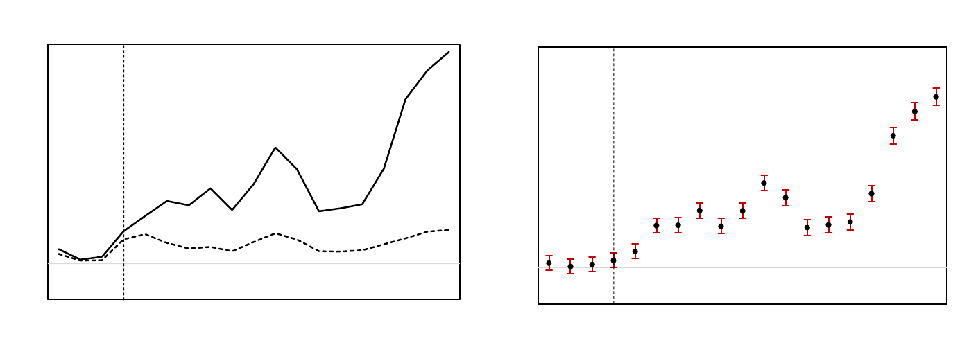
46
!
Figure 1: HARP and Refinancing Rate in Treatment and Control Groups
Panel (a) of the figure shows the percentage of loans refinancing around the HARP implementation in the treatment group (solid line) and the control group (dashed
line) in a given quarter. Panel (b) shows the estimated coefficients of interaction terms between quarterly time dummies and the treatment indicator (HARP Eligible)
along with 95% confidence intervals for the specification where the dependent variable takes the value of one whether the loan refinances (through HARP or
otherwise) in a given quarter and is zero otherwise. The refinanced loans exit the estimation sample. The specification is similar to one in Column (2) of Table 2A
but where we replace the After Q1 2009 dummy with a set of quarterly dummies. This specification allows us to investigate the quarter-by-quarter changes in the
refinancing rate between the treatment and control group (relative to the level in 2008:Q1). The vertical dashed line marks the beginning of the HARP program. Data
Source: Equifax-BKFS CRISM Data.
(a) Refinancing rate in the treatment and control group
(b) Differential change in the refinancing rate of HARP eligible loans
-1%
0%
1%
2%
3%
4%
5%
6%
2008q2
2008q3
2008q4
2009q1
2009q2
2009q3
2009q4
2010q1
2010q2
2010q3
2010q4
2011q1
2011q2
2011q3
2011q4
2012q1
2012q2
2012q3
2012q4
-1%
0%
1%
2%
3%
4%
5%
6%
2008q2
2008q3
2008q4
2009q1
2009q2
2009q3
2009q4
2010q1
2010q2
2010q3
2010q4
2011q1
2011q2
2011q3
2011q4
2012q1
2012q2
2012q3
2012q4

47
!
Figure 2: HARP and Durable (Auto) Consumption around Refinancing Date
Panel (a) of this figure plots the OLS estimates for quarterly time fixed effects (along with 95% confidence intervals) from the specification where the dependent
variable takes the value of one if a new auto financing transaction takes place in a given quarter and is zero otherwise. In this specification we include a set of controls
capturing borrower, loan, and regional characteristics and a set of (plotted) quarterly time dummies that capture the three quarters preceding HARP refinancing and
eight quarters following HARP refinancing date. Panel (b) shows the corresponding results for the specification with the net amount of new auto financing (in dollars)
as the dependent variable. Data Source: Data Source: Equifax-BKFS CRISM Data.
(a) Change in the probability of new auto financing
(b) Change in the net amount of new auto financing
-0.6%
-0.4%
-0.2%
0.0%
0.2%
0.4%
0.6%
0.8%
1.0%
1.2%
1.4%
1.6%
Q-3 Q-2 Q-1 Q1 Q2 Q3 Q4 Q5 Q6 Q7 Q8
-100
-50
0
50
100
150
200
250
300
350
Q-3 Q-2 Q-1 Q1 Q2 Q3 Q4 Q5 Q6 Q7 Q8

48
!
Figure 3: HARP and Durable (Auto) Consumption in Treatment and Control Groups
Panel (a) of the figure shows the quarterly new auto financing around the HARP implementation among borrowers in the treatment group (solid line) and the control
group (dashed line) in a given quarter. Panel (b) shows the estimated coefficients of the quarter-by-quarter changes in the new auto financing between the treatment
and control group (relative to the level in 2008:Q1) along with 95% confidence interval around these estimates. The specification is similar to one in Column (8) of
Table 2C but where we replace the After Q1 2009 dummy with a set of quarterly dummies. The vertical dashed line marks the beginning of the HARP program. Data
Sources: Equifax-BKFS CRISM Data.
(a) The net amount of new auto financing in the treatment and control groups
(b) Differential change in the new auto financing among HARP eligible
400
500
600
700
800
900
1000
1100
1200
2008q2
2008q3
2008q4
2009q1
2009q2
2009q3
2009q4
2010q1
2010q2
2010q3
2010q4
2011q1
2011q2
2011q3
2011q4
2012q1
2012q2
2012q3
2012q4
-200
-175
-150
-125
-100
-75
-50
-25
0
25
50
75
100
125
150
175
200
2008q2
2008q3
2008q4
2009q1
2009q2
2009q3
2009q4
2010q1
2010q2
2010q3
2010q4
2011q1
2011q2
2011q3
2011q4
2012q1
2012q2
2012q3
2012q4

49
!
Figure 4: HARP-Conforming Spread and the Fraction of Loans Refinanced by the Same Servicer across LTV
Panel (a) of this figure presents the OLS estimates for the LTV dummies of (80,90], (90, 105], (105, 125] and >125 along with 95% confidence interval from the
specification with the HARP spread relative to confirming refinances (in basis points) being the dependent variable. Panel (b) shows the estimates of the same
dummies from the specification with the dummy variable, Same Servicer, which takes the value of one if the loan is refinanced by the lender servicing the legacy
mortgage and is zero otherwise. The conforming refinances with LTV equal to 80 serve as the excluded category (33% of these loans are refinanced by the same
servicer). Other controls include the current FICO score (and its square) of the borrower and the metropolitan statistical area (MSA) fixed effects corresponding to
the location of the property, time fixed effects capturing the quarter/year time during which the loan was refinanced (Year-Quarter FEs), and the fixed effects
corresponding to the identity of the lender refinancing the loan (Servicer FEs). Standard errors are included in the parentheses. Data Source: Large secondary-market
participant.
(a) HARP-conforming refi spread (bps)
(b) Refinances by the Same Servicer (%)
10
15
20
25
30
35
40
(0.8, 0.9] (0.9, 1.05) [1.05,1.25) > 1.25
40
50
60
70
80
90
100
(0.8, 0.9] (0.9, 1.05) [1.05,1.25) > 1.25
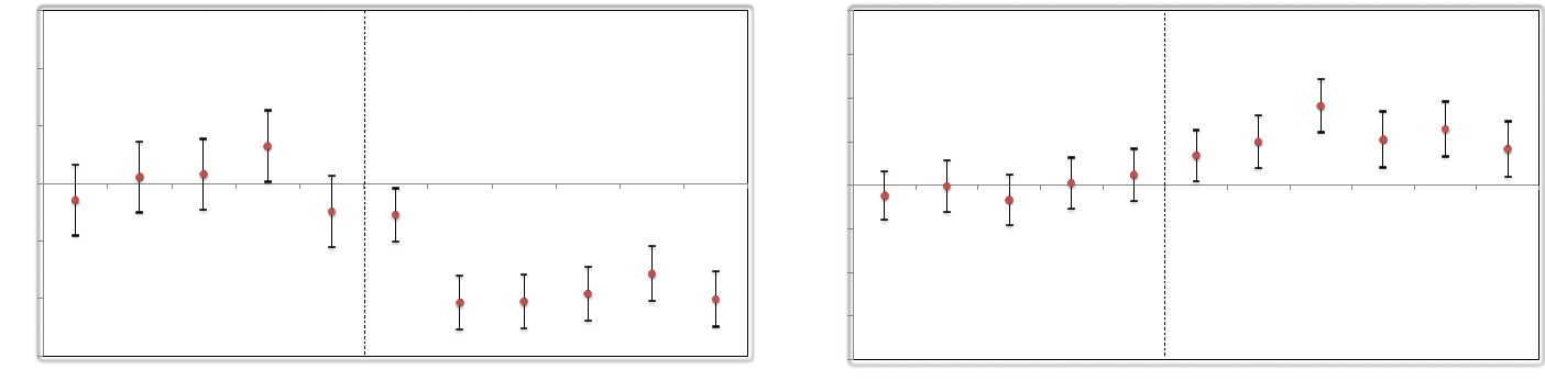
50
!
Figure 5: Change in the Program Rules and the HARP-Conforming Refinancing Spread and Rate
Panel (a) of this figure plots the estimated coefficients (based on OLS) for monthly fixed effects along with 99% confidence intervals around these estimates from a
regression of HARP-conforming refi spread (in basis points) on a set of borrower and loan characteristics including current loan LTV ratios, borrower credit scores,
servicer fixed effects, MSA fixed effects, previous rate, and monthly time fixed effects. The excluded category corresponds to HARP refinances that occurred during July
2012 so the plotted coefficients show the estimated change relative to the spread from this period. Panel (b) shows the corresponding results from the specification where
now the dependent variable takes the value of one if the loan refinances in a given month and is zero otherwise. The plotted coefficients are the estimated interaction terms
of time dummies with HARP eligible dummy. In panel (b) the base category are loans that are eligible for conforming refinances (loans with current LTV as of June 2012
less than 80). The displayed coefficients in panel (b) show the estimated change in the difference between refinancing rates of HARP and conforming loans (relative to
the level in July 2012). The estimation period is from July 2012 till June 2013. As we observe the HARP spread and the difference between refinancing rates of HARP
eligible and conforming loans generally persists at a stable level prior to the change in program rules in January 2013. Once the new rules are in place the spread declines
sharply by about 10 basis points in 2013 and the HARP refinancing rate experiences a significant differential increase (by about 0.12% per quarter).
!
(a) Change in the HARP-conforming spread
(b) Change in the refinancing rate
-15
-10
-5
0
5
10
15
Aug-12 Sep-12 Oct-12 Nov-12 Dec-12 Jan-13 Feb-13 Mar-13 Apr-13 May-13 Jun-13
-0.4%
-0.3%
-0.2%
-0.1%
0.0%
0.1%
0.2%
0.3%
0.4%
Aug-12 Sep-12 Oct-12 Nov-12 Dec-12 Jan-13 Feb-13 Mar-13 Apr-13 May-13 Jun-13

51
!
On-Line Appendix A: Additional Analysis
Appendix A1: HARP and the Refinancing Rate in the Matched Sample
Panel A presents summary statistics of key variables in the pre-HARP period (2008: Q2 to 2009: Q1) in the treatment and control groups. The treatment group
consists of GSE 30-year fixed-rate mortgages that have current LTV ratios greater than 80 as of March 2008 (one year prior to the program). The control group
consists of a sample of full documentation prime non-GSE 30-year fixed-rate mortgages (privately securitized) that have current LTV ratios greater than 80 as of
March 2008. Since, these loans were not sold to GSEs they are not eligible for HARP. These loans were further matched based on FICO credit scores of borrowers,
current LTV ratios, interest rates, and loan amounts. Panel B presents OLS estimates from regressions that track whether a loan refinances around the program
implementation (Q2 2008 till Q4 2012). The dependent variable takes the value of one in the quarter a given loan refinances and is zero otherwise (the refinanced
loans exit the estimation sample). The variable, HARP Eligible, takes the value of one if a loan belongs to the treatment group (HARP Eligible) and is zero otherwise.
The variable, After Q1 2009, takes the value of one for the quarters after Q1 2009 and is zero otherwise. Column (1) presents the basic specification with no other
controls but a constant term, HARP Eligible dummy, After Q1 2009 dummy, and the interaction term of these two variables (HARP Eligible) × After Q1 2009).
Column (2) adds borrower controls that include variables such as FICO credit score, LTV, interest rates, and Column (3) adds the fixed effects for the location (MSA)
of the property (MSA FEs). Standard errors are included in the parentheses. Data Source: Large secondary-market participant and BlackBox Logic.
Panel A: Summary statistics (matched sample)
Panel B: HARP and the refinancing rate
Treatment
(HARP Eligible)
Control
(Non-HARP Eligible)
Mean
(1)
S.D
(2)
Mean
(3)
S.D
(4)
LTV
95.5
5.2
95.6
5.8
FICO
727.7
46.4
728.4
43.7
Interest Rate
6.60
0.64
6.62
0.66
Balance
183,614
91,718
186,525
110,104
Number of Loans
46,154
46,154
(1)
(2)
(3)
(HARP Eligible) × After Q1 2009
1.73
(0.05)
1.35
(0.07)
1.37
(0.07)
Borrower Controls
No
Yes
Yes
MSA FEs
No
No
Yes
Observations
1,372,731
1,372,731
1,372,731
Adjusted R-Square
0.001
0.003
0.01

52
!
Appendix A2: Cumulative Change in the Durable Spending (New Auto Financing) after the HARP Refinancing Date
Panel (a) shows the estimated cumulative change in the net amount of new auto financing (in dollars) along with 99% confidence intervals in the eight quarters
following the HARP refinancing. These estimates are from a borrower level specification where the dependent variable is the net amount of new auto financing in
dollars. We include a set of controls capturing borrower, loan, and regional characteristics and a set of quarterly time dummies that capture the three quarters
preceding HARP refinancing and eight quarters following HARP refinancing date. Panel (b) plots the estimates for less indebted borrowers with below median LTV
(dashed line) and more indebted borrowers with above median LTV (solid line). The average differences across these groups in Panels (b) are statistically significant
at 1%.
(a) Cumulative change in the new car spending after HARP refinance
(b) New car spending among less/more indebted (below/above median LTV)
!
!
!
!
!
!
-200
0
200
400
600
800
1000
1200
1400
1600
1800
2000
Q-3 Q-2 Q-1 Q1 Q2 Q3 Q4 Q5 Q6 Q7 Q8
0
200
400
600
800
1000
1200
1400
1600
1800
2000
Q1 Q2 Q3 Q4 Q5 Q6 Q7 Q8

53
!
Appendix A3: Origination Leverage and the Borrower’s Creditworthiness among Agency and Non-Agency Loans
This figure tracks the evolution of average FICO credit scores (panel a) and LTV ratios (panel b) of borrowers obtaining prime conventional FRM loans by origination
month during 2003-2007 period. The solid line shows these statistics for the agency loans while the dashed line shows the corresponding evidence for non-agency
loans. The sample is restricted to borrowers who downpay at least 20% of home value, have loan balances below the conforming loan limit, and have the initial LTV
ratios greater than 60%. The figure stops in the first quarter of 2007 as there were very few non-agency FRM loans originated after that period due to the collapse of
private label loan market (except of the jumbo market).
(a) FICO credit score
(b) LTV
350
400
450
500
550
600
650
700
750
800
850
Jan-03
Apr-03
Jul-03
Oct-03
Jan-04
Apr-04
Jul-04
Oct-04
Jan-05
Apr-05
Jul-05
Oct-05
Jan-06
Apr-06
Jul-06
Oct-06
Jan-07
0
10
20
30
40
50
60
70
80
90
100
Jan-03
Apr-03
Jul-03
Oct-03
Jan-04
Apr-04
Jul-04
Oct-04
Jan-05
Apr-05
Jul-05
Oct-05
Jan-06
Apr-06
Jul-06
Oct-06
Jan-07

54
!
Appendix A4: Pre-Trends: Refinancing Rate and Auto Consumption in Treatment and Control Groups
Panel (a) shows the estimated coefficients of interaction terms between quarterly time dummies and the GSE loan dummy along with 95% confidence intervals for
the specification where the dependent variable takes the value of one whether the loan refinances in a given quarter and is zero otherwise. The refinanced loans exit
the estimation sample. Panel (b) shows the estimated coefficients of interaction terms between quarterly time dummies and the GSE loan dummy along with 95%
confidence intervals for the specification where the dependent variable is the new auto financing. The sample consists of prime conforming GSE and non-agency
FRM mortgages with balances below the conforming loan limit that were outstanding as of the beginning of 2006. The estimation period covers two years preceding
our main estimation sample (2006:Q1 to 2008:Q1). To facilitate comparison with the corresponding effects during the program both figures have the same scale as
corresponding panels in Figure 1 and 3. Data Source: Equifax.
(a) Refinancing rate
(b) New auto cosnumption
-1%
0%
1%
2%
3%
4%
5%
6%
2006q2 2006q3 2006q4 2007q1 2007q2 2007q3 2007q4 2008q1 2008q2
-200
-175
-150
-125
-100
-75
-50
-25
0
25
50
75
100
125
150
175
200
2006q2 2006q3 2006q4 2007q1 2007q2 2007q3 2007q4 2008q1 2008q2

55
!
Appendix A5: Geographical Distribution of Zip Codes and HARP Eligible Share
This figure presents the geographic distribution of zip codes in our overall sample across the United States. In addition, the figure displays the fraction of loans in a
zip code which are eligible for HARP (as of March 2009). As we observe, there is a significant variation in the HARP Eligible share across zip codes (ranging from
just few percent of loans being eligible for the HARP program to more than 70%). Data Sources: Equifax-BKFS CRISM Data.
!
!

56
!
Appendix A6: Program Refinancing Rate, Mortgage Rate Reduction, and the Fraction of Eligible Loans and Eligible Loans
Serviced by High Cost Lenders in a Zip Code
Column (1) and (2) of this table investigates the relation between the fraction of loans in a zip code refinancing under HARP as the dependent variable and zip code
level Eligible Share and Eligible and High Cost Servicer Share. Eligible Share is the fraction of loans in a zip code that are GSE and have current LTV ratios greater
than 80 prior to the program implementation. Eligible and High Cost Servicer Share is the fraction of loans in a zip code that are GSE, have current LTV ratios
greater than 80 and are serviced by high cost servicers prior to the program implementation. We also include a set of controls including the zip code average FICO
credit score, LTV ratio, interest rate on mortgages along with the average zip code house price growth over the prior five years and state fixed effects. Column (1)
presents the specification without Eligible and High Cost Servicer Share control, while Column (2) repeats this analysis, but includes this variable in the set of
controls. Columns (3) and (4) provide the corresponding analysis for the reduction in the average mortgage rate in a zip code (in basis points) during first four years
of the program and zip code level Eligible Share and Eligible and High Cost Servicer Share. The servicer is classified as high cost if it is in the top quartile of
servicers with the highest estimated fixed effects as displayed in Appendix A7. These high cost servicers account for over 60% of loans in our data. Standard errors
(based on the OLS estimates) are included in parentheses.
Dependent variable:
Fraction of loans in a zip code
refinancing under HARP
Dependent variable:
Reduction in the average mortgage
interest rate in a zip code
(in basis points)
(1)
(2)
(3)
(4)
HARP Eligible Share
0.24
(0.01)
0.35
(0.01)
38.0
(0.01)
49.1
(0.03)
Eligible and High Cost Servicer Share
-
-0.16
(0.03)
-
-17.4
(0.05)
Zip Code Controls
Yes
Yes
Yes
Yes
State FEs
Yes
Yes
Yes
Yes
Adj. R-squared
0.68
0.69
0.70
0.71

57
!
Appendix A7: Regional Outcomes and Harp Eligible Share
This table examines the relation between regional (zip code level) consumer credit card spending, durable (auto spending), foreclosures, and house prices and the
HARP Eligible Share. The HARP Eligible Share, is the fraction of outstanding first-lien GSE mortgage loans in a zip code that have current LTV ratios greater than
80 prior to the program implementation. Columns (1) and (2) show the results for the change in the quarterly credit card spending growth rate, Columns (3) and (4)
the auto purchase growth rate, Columns (5) and (6) for the foreclosure rate, and Columns (7) and (8) for the house price growth rate, all computed as the average of
the respective value during the program (after 2009:Q1) less its pre-program level (average during 2008:Q1 to 2009:Q1 period). Standard errors are included in
parentheses. Data Sources: Black Knight Data and Analytics, Polk, Zillow, Corelogic, Equifax.
Credit Card Spending
Auto Purchase Growth
Foreclosure Rate
House Prices
(1)
(2)
(3)
(4)
(5)
(6)
(7)
(8)
HARP Eligible
0.148
0.173
0.498
0.272
-0.003
-0.008
0.111
0.046
(0.035)
(0.056)
(0.023)
(0.031)
(0.001)
(0.001)
(0.003)
(0.002)
Other Controls
No
Yes
No
Yes
No
Yes
No
Yes
State FE
No
Yes
No
Yes
No
Yes
No
Yes
Observations
2816
2816
2816
2816
2816
2816
2816
2816
Adjusted R-squared
0.006
0.040
0.135
0.444
0.006
0.707
0.229
0.881
!

58
!
Appendix A8: Credit Card Spending, Auto Purchase, and House Price Growth in High and Low HARP Exposed Areas
This figure shows the average credit card spending, auto purchase, and house price growth rates in the high HARP exposed (above median Eligible Share) and low
HARP exposed (below median Eligible Share) zip codes. The high HARP exposed group is displayed in solid line and low HARP exposed group is displayed in
dashed line. Zip code credit card spending growth is computed using proprietary data from U.S. Treasury. The auto purchase growth data come from Mian and Sufi
(2010) (based on R.L. Polk & Company data). The house price growth is computed using CoreLogic zip-code level price indices.
(a) Credit card spending growth
(b) Auto purchase growth
(c) House price growth
-15%
-10%
-5%
0%
5%
10%
15%
20%
2009 2010 2011 2012 2013
-25%
-20%
-15%
-10%
-5%
0%
5%
10%
15%
20%
25%
2008 2009 2010 2011 2012 2013
-10%
-8%
-6%
-4%
-2%
0%
2%
4%
6%
8%
2008q1
2008q2
2008q3
2008q4
2009q1
2009q2
2009q3
2009q4
2010q1
2010q2
2010q3
2010q4
2011q1
2011q2
2011q3
2011q4
2012q1
2012q2
2012q3
2012q4
2013q1
2013q2
2013q3
2013q4

59
!
Appendix A9: HARP-Conforming Spread across Lenders
Panel (a) of this figure plots the servicer fixed effects corresponding to the identity of HARP lender from the specification in Column (2) of Table 5, in which the
dependent variable is the HARP-conforming refi spread along with 95% confidence intervals. Lender names have been anonymized. Panel (b) shows the relation
between the lenders’ fixed effects (y-axis) and their log asset size as of 2009 (x-axis). This figure is plotted only for the lenders for which we have asset size data
collected from publicly available sources. Data Source: Large secondary-market participant.
(a) Lenders’ fixed effects
(b) Lender’s fixed effects and log asset size
-40
-35
-30
-25
-20
-15
-10
-5
0
5
10
15
20
25
1 2 3 4 5 6 7 8 9 10 11 12 13 14 15 16 17 18 19 20 21 22 23 24 25 26 27 28 29 30 31 32 33 34 35 36 37 38 39 40 41 42 43 44 45 46 47 48
-25
-20
-15
-10
-5
0
5
10
15
20
25
8 9 10 11 12 13

60
!
Appendix A10: Evolution of Observables among HARP and Conforming Refinances prior to the Program Change
This figure tracks the evolution of average FICO credit scores (panel a) and LTV ratios (panel b) of borrowers at the time of loan refinancing among HARP and
conforming refinance during the six months preceding the change in the program rules. The solid line represents HARP refinances while the dashed line shows the
corresponding means for conforming refinances. The average LTV ratio for HARP refinances consistently remains about 30% above that for conforming refinances,
with little relative change over time (by construction our benchmark conforming refinances have LTV ratios equal to 80 percent). We do not observe a substantial
relative variation in the borrower credit scores between HARP and conforming refinances.
(c) FICO credit score
(d) LTV
350
400
450
500
550
600
650
700
750
800
850
2012-Jul 2012-Aug 2012-Sep 2012-Oct 2012-Nov 2012-Dec
0
20
40
60
80
100
120
140
2012-Jul 2012-Aug 2012-Sep 2012-Oct 2012-Nov 2012-Dec

61
!
Appendix A11: Quantitative Life-Cycle Model: The Effect of HARP on Consumption and Welfare of Eligible Borrowers
This table shows an annual increase in the household consumption in 1000s of dollars in the first 3 years of the program relative to the world without HARP (Panel
A) and the welfare gains due to HARP to borrowers as a percentage of the borrower’s lifetime utility (Panel B) in the cross-section of borrowers based on their
current LTV and their pre-refinance mortgage rate. These results are calculated based on the model simulations from Section VI assuming the borrower can refinance
to an average mortgage rate of 4.5% plus the monopolistic markups from Table 4B. Panel C shows additional welfare gains as a percentage of the borrower’s lifetime
utility that arise by eliminating the HARP interest rate markups.
Pre-refinance mortgage rate
5.5%
6.0%
6.5%
7.0%
LTV
Panel A: Consumption response to HARP (annual average over 3-year period)
(0.8, 0.9]
0.60
0.96
1.24
1.53
(0.9, 1.05)
0.64
1.09
1.61
1.91
[1.05,1.25)
1.03
1.37
1.85
2.31
> 1.25
1.12
1.76
2.38
2.87
Panel B: Utility gain from HARP (% of lifetime utility)
(0.8, 0.9]
0.37
0.47
0.66
0.79
(0.9, 1.05)
1.08
2.04
4.76
6.53
[1.05,1.25)
2.01
4.66
9.86
13.45
> 1.25
2.76
6.13
12.53
16.32
Panel C: Utility gain from elimination of HARP markups (% of lifetime utility)
(0.8, 0.9]
0.22
0.22
0.37
0.46
(0.9, 1.05)
0.30
0.30
0.54
0.61
[1.05,1.25)
0.57
0.55
0.98
1.07
> 1.25
0.85
0.83
1.33
1.50

62
!
Appendix A12: Impact of HARP Markups on Consumption and the Refinancing Rate of Eligible Borrowers
Panel A of this figure shows an average increase in the borrower’s annual consumption due to HARP during the first 3 years relative to the world without HARP in
the cross-section of borrowers based on their current LTV. These results are calculated based on the model simulations from Section VI for the borrower with an
average prior rate of about 6% who can refinance to an average rate of 4.5% plus the monopolistic markups from Table 4B in the case of HARP with markups. These
rates correspond to the mean rates in in our sample for HARP borrowers. Panel B shows the percentage of borrowers who refinance their loans during the first three
years based on the optimal refinancing function implied by our model from Section VI applied to a random sample of borrowers that were eligible for HARP as of
its implementation date in March 2009. This sample amounts to more than 1.1 million conforming mortgages from a large secondary market participant, which is
more than 15% of the entire population of eligible loans. Top black solid line shows the case in which borrowers can refinance (at no additional cost) to the benchmark
conforming rate (with no guarantee fees). The middle solid gray line shows the case in which borrowers face the HARP guarantee fees. The bottom dashed gray line
(in panel b) shows the case in which there is no HARP.
(a) Borrower’s consumption increase due to HARP (annual in $)
(b) Refinancing rate among HARP eligible borrowers (in %)
$600
$800
$1,000
$1,200
$1,400
$1,600
$1,800
$2,000
$2,200
(0.8, 0.9] (0.9, 1.05] (1.05, 1.25] >1.25
HARP with markups
HARP with no markups
LTV
0%
10%
20%
30%
40%
50%
60%
70%
80%
90%
100%
(0.8, 0.9] (0.9, 1.05] (0.9, 1.05] >1.25
HARP with markups
HARP with no markups
No HARP
LTV

63
!
On-Line Appendix B:
Variation in HARP-Conforming Refi Spread and Legacy Interest Rate
This appendix provides more discussion of our conjecture that the legacy interest rate on the
mortgage prior to refinancing may be systematically related to the degree of pass-through under
HARP. To see this argument further, consider the simple example where two similar HARP eligible
borrowers (A and B) want to refinance their loans. The interest rates on their original loans (i.e., the
legacy interest rates) are R
A,0
and R
B,0
, such that R
A,0
> R
B,0
. Given the assumed similarity of
borrower’s risk characteristics, the difference in interest rates faced by the borrowers could reflect
time variation in benchmark risk-free rates pinned down by the timing of when these borrowers
obtained their original loans. We further assume that a borrower needs to obtain a reduction of the
interest rate of at least Δ per year in order to refinance a loan (see Agarwal, Driscoll, and Laibson
(2013) for an optimal rule for Δ). An existing lender requires an interest rate of R
even
to break even
on the new mortgage, given the borrower’s risk characteristics. Since by assumption, borrowers A
and B have identical risk profiles at the time of refinancing, they face the same breakeven rate. In a
perfectly competitive market – proxied in our benchmark analysis by the conforming refinancing
market -- the same R
even
would apply to all lenders. However, suppose a new lender must charge a
rate premium, δ, to compensate for higher underwriting costs due to higher put back risk (Section
II). In this setting, what interest rates could be obtained by A and B on their respective loans? The
diagram below sketches out the case for borrower A.
The shaded area represents the region of rates that satisfy the participation constraints of both the
borrower and the lender. Although the existing lender can potentially charge R
A,0
– Δ, the presence
of the outside option offered by the new lender effectively constrains the maximum rate offered by
the existing lender to be R
even
+ δ. This results in the existing lender being able to charge an interest
rate above the expected cost and extracting some surplus from the borrower.
In the case of borrower B, the existing loan has a lower interest rate, although it is still higher than
the rate on the newly refinanced loan. In the diagram below, a new lender is unable to offer a rate
R
even
+δ as this rate does not satisfy the borrower’s participation constraint. However, because (R
B,0
– Δ) < (R
even
+ δ), the existing lender can still realize a markup over its expected cost of funding the
loan, albeit smaller than in the case of Borrower A. This difference in the interest rates obtained by
A and B occurs despite the fact that these borrowers have the same risk characteristics.
Interest rate
R
A,0
R
A,0
-Δ
R
even
+δ
R
even

64
!
The discussion above assumes that the current lender (servicer) knows the borrower’s participation
constraint as well as the costs of other lenders. In reality the incumbent lender may be imperfectly
informed about both the borrower’s participation constraint as well as the refinancing cost structure
of its competition (i.e., the incumbent lender may only know distributions of these factors). In such
a scenario, the decision of the incumbent lender regarding the rate to be offered will reflect the trade-
off between the expected profit in the case that the offer is accepted versus the risk of losing the
borrower either due to violating the borrower participation constraint (offering insufficient reduction
in rate) or due to other lenders being able to offer a lower rate (if their refinancing cost proves to be
low enough).
It is not difficult to construct a simple market equilibrium model featuring such a tradeoff. In such
equilibrium, consistent with the above discussion, the incumbent lender will still offer higher
refinancing rates to borrowers with higher legacy rates and to borrowers for whom the expected cost
of refinancing by other lenders is larger (and hence there is less competition). Moreover, fewer
borrowers will end up refinancing their loans relative to the case when the incumbent servicer would
offer its zero profit rates. These borrowers would be the ones with required reduction in rates higher
than the one offered by the incumbent lender but lower than what is implied by a break-even rate.
In addition, some loans will also be refinanced by other non-incumbent lenders (i.e., mortgages they
can refinance at relatively low refinancing costs).
Interest rate
R
B,0
R
B,0
-Δ
R
even
+δ
R
even
65
!
On-Line Appendix C:
Life-Cycle Model of Refinancing and Consumption
In this Appendix we develop a life-cycle model of refinancing that quantitatively rationalizes these
empirical patterns and helps evaluate welfare effects of altering the refinancing market by removing
the housing equity eligibility constraint, like HARP did, and lowering competitive frictions.
We consider a setting where a household lives for a finite number of discrete life-cycle periods,
!"
#$%$&
, with a probability of survival from period
!'(')
to
!
of
*
!
, and
*
&
= 0. Calendar time is
indexed by
+
, with periods of the same length as the life-cycle periods; household age in calendar
period
+
is denoted by
!
+
. Every period until retirement at age
!
,
, the household receives labor
income
-
+
.!
+
/
that follows an exogenous stochastic process. After retirement, the household
receives a constant fraction of its last labor income
-
+
.!
,
/
until death. The household chooses
consumption of housing services
0
+
and other goods
1
+
(the numéraire) every period to maximize
expected lifetime utility. The per-period utility function
2.1
+
$0
+
/
is assumed to satisfy the usual
properties of being strictly increasing and concave in its two arguments arguments. Lifetime utility
at age
!
+
'
"'#
is given by
3
4
56
7
4
8
49:
;
<
=
>
?
=
>@A
2
.
1
4
$0
4
/
B<
=
>
.)(?
=
>@A
/C
4
D
'
E
'$
where
C
+
is the bequest the household leaves to its children in case it does not survive until period
+B)
, and
<
=
>
"
F
?
=
G
4
H9:
is the unconditional probability that the household is alive in period
+'I
'&
.
A house of size
J
4
produces housing services with the linear technology
0
+
'
"'J
+
. A unit of the
housing asset sells for price
K
4
. In addition to the housing asset, the household can save the amount
L
+
in a risk-free bond. The household can also borrow an amount
M
+
'
in mortgage debt. The market
interest rate for new mortgage contracts in period
+
(“market rate”) is given by the combination of
the short-term risk free rate
N
4
plus a mortgage spread
O
:
N
4
P
"N
4
BOQ
In order to borrow, the household has to own a house and use part of its value as collateral. In
particular, when the household buys a house, it can at most borrow an amount
.)'('R
S
/'
of the
house value to finance the purchase, where
R
S
is the fraction required as a down payment:
M
4
T.)(R
S
/K
4
J
4
At the time of the house purchase, the household needs to pay a mortgage closing fee proportional
66
!
to the mortgage principal,
UM
4
. The contract fixes the current market rate and the initially chosen
mortgage principal for the duration of the mortgage. The mortgage principal amortizes at a fixed
rate of
R
P
. Further, mortgage interest payments are deductible from taxable income at a marginal
tax rate of
V
W
. We assume that houses are illiquid, and that selling a house requires a transaction cost
X
that is proportional to the value of the house. The effective proceeds from selling a house of size
J
4
in period
+
are hence
.)'('X/'K
4
J
4
.
We assume individual household income is given by
-
4$Y
"-
Z
4
-
[
4
8
\]^
_
`
_
!
4$Y
a
Bb
4$Y
a
$
where
-
Z
4
is the level of aggregate per-capita income growing at deterministic rate
c
,
-
Z
4
"-
Z
4de
\]^
.
c
/
$
and
-
[
4
8
is the cyclical component of aggregate income with mean one. Both
`
_
!
4$Y
a
and
b
4$Y
are
idiosyncratic income components:
b
4$Y
is a mean-zero income shock and
`
_
!
4$Y
a
is the deterministic
age-specific mean income. Idiosyncratic income shocks are persistent and follow an AR(1) process
at the level of the individual household
b
4$Y
"'X
f
b
4de$Y
B'g
4
f
$
where
g
4
f
is i.i.d. with mean zero and standard deviation
h
f
. Similarly, house prices follow the
process:
K
4
"K
Z
-
Z
4
K
[
4
8
$
where
K
Z
is a constant determining the scale of house prices relative to trend GDP, and
K
[
4
8
is the
cyclical component of house prices with mean one. Given our assumption on preferences and the
partial equilibrium setting, only housing expenditure matters from the perspective of household
optimization. Therefore,
K
Z
is merely a normalization.
Together with the cyclical components of income and house prices, the risk free savings rate follows
a first-order vector autoregressive process (VAR). Denote the vector containing three aggregate
state variables as
i
4
"'
j
-
[
4
8
$K
[
4
8
$N
4
'
k
l
Q
Then
mno'.i
4
/"&BCmno'.i
4de
/Bg
4
'
,
where
&
is a 3x1 vector and
C
is a 3x3 matrix of coefficients, and
g
4
is a 3x1 vector of mean-zero
innovations with variance-covariance matrix
p
.
We use power utility with coefficient
q
and a Cobb-Douglas aggregator over nondurable and

67
!
housing consumption:
2
.
1
4
$J
4
/
"'
r
s
>
Atu
S
>
u
v
Atw
edx
.
The Cobb-Douglas exponent
y
parameterizes optimal housing expenditure. For the bequest motive,
we adopt the functional form
C
.
z
4
B-
4
/
"'C
Z
.
.{
>
|}
>
/~
Z
tu
/
Atw
edx
.
Bequest utility has the same power form in total wealth as regular utility. Parameter
C
Z
'
determines
the strength of the bequest motive. Similarly, for the utility penalty of defaulting households, we
assume
•
.
z
4
B-
4
/
"'€
.
.{
>
|}
>
/~
Z
tu
/
Atw
edx
,
with
€
determining the magnitude of the penalty.
We can summarize terms of a mortgage contract that a household has obtained in some previous
period by the remaining mortgage balance and the “locked-in” mortgage rate. To describe the
decision problem of the household, it is useful to distinguish the following cases.
1. The household always has the option of staying in the current house and keeping the same
mortgage terms, while either staying on the fixed amortization schedule or prepaying part of the
mortgage balance. This means the mortgage rate going into next period stays fixed.
2. The second option is to stay in the current house, but refinance the mortgage at the current market
rate. In this case, the closing fee needs to be paid. In the absence of HARP, in order to refinance,
households need to satisfy the housing equity constraint: the LTV ratio of the new loan with
respect to the current market value of the house cannot exceed 80%. Consequently, households
who experienced a sufficient decline in their home values are ineligible for refinancing unless
they save enough to deleverage. Introduction of HARP is equivalent to removal of this
refinancing eligibility constraint.
3. The third option is to buy a new house and obtain a new mortgage at the market rate. In this case,
the closing fee needs to be paid and the down payment requirement is enforced with respect to
the value of the new house.
4. Finally, the household can choose to default on its mortgage. In this case, the mortgage debt is
erased, the house is seized by the mortgage lenders, and the household has to rent for its remaining
life. Further, the household incurs a one-time additive utility penalty that is an increasing function
of household wealth.

68
!
We do not include the option to sell the current house and instead rent. Despite the general potential
of a rental option to mitigate the severity of borrowing constraints in the mortgage market (Kaplan
et al (2017)), we do not believe that the option to sell and rent is quantitatively important for
evaluating the benefits of HARP. The home owners who are most likely to benefit from HARP are
those with significantly negative home equity. Absent HARP, these home owners usually face the
choice between either staying in their house and paying off their mortgage, or defaulting on their
mortgage and renting. The option to sell the house and move to the rental market is as infeasible as
refinancing for these borrowers with substantially negative home equity.
For brevity, we leave a formal statement of the value functions to Appendix C, which also discusses
in detail the numerical solution of the model. Our benchmark calibration strategy is as follows. The
housing related parameters are set to common values in the literature on housing markets that
represent long-run estimates. We calibrate the remaining preference parameters to match data
moments from the 2010 Survey of Consumer Finances (SCF). To determine the coefficients of the
VAR for the exogenous state variables, we estimate a VAR on the GDP per capita, a price index
based on private residential fixed investment and one-year treasury yields, all annual for the period
1954-2016. More details are provided in Appendix Section C.4.
Figure C.1 in Appendix C shows that the model does a good job of replicating the patterns of the
average wealth-to-income and house value-to-income ratios in the cross-section of households in
the 2010 SCF.
33
Overall, the model provides a close enough fit to the data that we are comfortable
using it to assess the counterfactual effects of altering the refinancing market.
!
!!!!!!!!!!!!!!!!!!!!!!!!!!!!!!!!!!!!!!!!!!!!!!!!!!!!!!!
!
33
As is common in life-cycle models with housing and mortgage choice, the model somewhat overstates leverage of
old households relative to the data.
69
!
On-Line Appendix D:
Life-Cycle Model Solution Algorithm and Parametrization
D.1 Model Setup
Denote the terms of the mortgage contract at the beginning of period
+
that a household has obtained
in some previous period by
.M
•
4
$N
‚
4
P
/Q
Further, denote the size of house owned at the beginning of
+
by
J
•
4
and the savings in risk-free debt by
L
Z
4
. To describe the decision problem of the household, it
is useful to distinguish five cases.
The household always has the option of staying in the current house and keeping the same mortgage
terms, while either staying on the fixed amortization schedule or prepaying part of the mortgage
balance. The mortgage debt for next period then has to satisfy
M
4
T.)(R
P
/M
•
4
, and the rate for
next period is
N
‚
4|e
P
=
N
‚
4
P
. The other choices are consumption
1
4
'
and savings
L
4
. The budget
constraint is
-
4
B
.
)BN
4de
/
L
Z
4
(.)B.)(V
W
/N‚
4
P
)'M
•
4
'='1
4
BL
4
BM
4
.
(4)
The second option is to stay in the current house, but refinance the mortgage at the market rate, such
that
N
‚
4|e
P
=
N
4
BO
. In this case, the closing fee needs to be paid and the down payment requirement
is enforced, i.e.
M
4
T.)(R
S
/K
4
J
•
4
. The budget constraint is
-
4
B
.
)BN
4de
/
L
Z
4
(.)B.)(V
W
/N‚
4
P
)'M
•
4
'='1
4
BL
4
(.)(ƒ/M
4
.
(5)
The third option is to buy a new house and obtain a new mortgage at the market rate, such that
N
‚
4|e
P
=
N
4
BO
. In this case, the closing fee needs to be paid and the down payment requirement is enforced
with respect to the value of the new house, i.e.
M
4
T.)(R
S
/K
4
J
•
4
. The budget constraint is
-
4
B
.
)BN
4de
/
L
Z
4
B
.
)(X
/
K
4
J
•
4
(.)B.)(V
W
/N‚
4
P
)'M
•
4
'='1
4
BL
4
BK
4
J
4
(.)(ƒ/M
4
.
(6)
Finally, the household can choose to default on its mortgage. In this case, the mortgage debt is
erased, the house is seized by mortgage lenders, and the household has to rent for its remaining life.
Further, the household incurs a one-time additive utility penalty that is an increasing function of
household wealth
•.z
4
B-
4
/
. The budget constraint is
-
4
B
.
)BN
4de
/
L
4de
'='1
4
BL
4
B„K
4
J
4
,
(7)
where
„
is the rent-to-price ratio.
D.2 Dynamic Program
We can define the liquid wealth of a household (assuming a hypothetical sale of its house) as
z
4
"
.
)(X
/
K
4
J
•
4
B
.
)BN
4de
/
L
Z
4
(.)B
.
)(V
W
/
N
‚
4
P
/M
•
4
.
Denote by
…
=
>
†
.z
4
$J
•
4
$M
•
4
$N
‚
4
P
$-
4
‡'i
4
/
the value function of a household with age
!
4
conditional on
the decision to stay and keep the same mortgage or prepay part of the balance (options 1 or 2), by
…
=
>
†ˆ
.z
4
$J
•
4
$-
4
‡'i
4
/
the value function conditional on the decision to stay and refinance (option 3),
and by
…
=
>
‰
.z
4
$-
4
‡'i
4
/
the value function conditional on the decision to sell the current house and
70
!
buy a new one (option 4).
To model default, denote by
…
=
>
ˆ
.z
4
$-
4
‡'i
4
/
the value function of a renting household with savings
z
4
. Renting households solve
…
=
>
ˆ
.
z
4
$-
4
‡'i
4
/
"*
=
>@A
Š
‹Œ•
s
>
$Ž
>
$S
>
2
.
1
4
$J
4
/
B'73
4
;
…
=
>@A
ˆ
.z
4|e
$-
4|e
‡'i
4|e
/
D•
B
_
)(*
=
>@A
a
C.z
4
B
-
4
)
subject to
z
4
B-
4
"1
4
BL
4
B„K
4
J
4
z
4|e
".)BN
4
/L
4
.
This implies that the optimization problem of a household conditional on the decision to default this
period is given by
…
=
>
•
.
z
4
•
$-
4
‡'i
4
/
"…
=
>
ˆ
.
z
4
•
$-
4
‡'i
4
/
(*
=
>@A
•.z
4
B-
4
).
where we defined wealth after default as
z
4
•
".)BN
4de
/L
Z
4
.
The value function of a household who has not previously defaulted is then
…
=
>
.
z
4
$J
•
4
$M
•
4
$N
‚
4
P
$-
4
‡'i
4
/
"‹Œ•'‘…
=
>
†
.
z
4
$J
•
4
$M
•
4
$N
‚
4
P
$-
4
‡'i
4
/
$…
=
>
†ˆ
.z
4
$J
•
4
$-
4
‡'i
4
/
,
…
=
>
‰
.z
4
$-
4
‡'i
4
/
,
…
=
>
•
.
z
4
•
$-
4
‡'i
4
/
’'Q
We will now define the optimization problems conditional on the different discrete decision options.
For households who stay and keep the same mortgage rate we get
…
=
>
†
.
z
4
$J
•
4
$M
•
4
$N
‚
4
P
$-
4
‡'i
4
/
"*
“
>@A
Š
‹Œ•
s
>
$Ž
>
$P
>
2
.
1
4
$J
•
4
/
B73
4
;
…
=
>@A
.z
4|e
$J
•
4
$M
4
$N
‚
4
P
$-
4|e
‡'i
4|e
/
D•
B
_
)(*
=
>@A
a
C.z
4
+
-
4
)
subject to
M
4
T.)(R
P
/M
•
4
z
4
B-
4
B^K
4
J
•
4
"1
4
BL
4
BK
4
J
•
4
(M
4
,
z
4|e
"
.
)(X
/
K
4|e
J
•
4
B.)BN
4
/L
4
(.)B
.
)(V
W
/
N
‚
4
P
/M
4
.
For households who stay and refinance we get
…
=
>
†ˆ
.
z
4
$J
•
4
$-
4
‡'i
4
/
"*
=
>@A
Š
‹Œ•
s
>
$Ž
>
$P
>
2
.
1
4
$J
•
4
/
B73
4
;
…
=
>@A
.z
4|e
$J
•
4
$M
4
$N
4
BO$-
4|e
‡'i
4|e
/
D•
B

71
!
_
)(*
=
>@A
a
C.z
4
B-
4
)
subject to
M
4
T.)(R
S
/K
4
J
•
4
z
4
B-
4
BXK
4
J
•
4
"1
4
BL
4
BK
4
J
•
4
(.)(ƒ/M
4
,
z
4|e
"
.
)(X
/
K
4|e
J
•
4
B.)BN
4
/L
4
(.)B
.
)(V
W
/
.N
4
B
O//M
4
.
For households that buy a new house we get
…
=
>
‰
.
z
4
$-
4
‡'i
4
/
"*
“
>@A
Š
‹Œ•
s
>
$Ž
>
$P
>
S
>
2
.
1
4
$J
4
/
B73
4
;
…
=
>@A
.z
4|e
$J
4
$M
4
$N
4
BO$-
4|e
‡'i
4|e
/
D•
B
_
)(
*
=
>@A
a
C.z
4
B-
4
)
subject to
M
4
T.)(R
S
/K
4
J
4
z
4
B-
4
"1
4
BL
4
BK
4
J
4
(.)(ƒ/M
4
,
z
4|e
"
.
)(X
/
K
4|e
J
4
B.)BN
4
/L
4
(.)B
.
)(V
W
/
.N
4
BO//M
4
.
Our assumptions on utility functions and stochastic processes allow us to define a transformed
stationary optimization problem by normalizing choice variables and value functions by trend
income. To do so, we first define transformed choice variables
”
+
'
"'1
+
•-
Z
4
,
–
+
'
"'L
+
•-
Z
4
and
—
+
'
"
'M
+
•-
Z
4
, and state variables
˜
+
'
"'z
+
•-
Z
4
and
—
•
4
"M
•
4
•-
Z
4
. We further define housing choice and
state variables in terms of expenditure at the trend house price as
™
4
"
~
Z
}
Z
>
S
>
}
Z
>
"K
Z
J
4
$™
Z
4
"
~
Z
}
Z
>
S
•
>
}
Z
>
"K
Z
J
•
4
.
Individual household income normalized by permanent income is
š
4
"
}
>
}
Z
>
"-
[
4
8
\]^
.
`
.
!
4
/
Bb
4
/
.
We can then write transformed optimization problems that define value functions
ƒ
=
>
›
.
œ‡N
4
/
"
•
ž
>
Ÿ
.
œ‡
>
/
.
}
Z
>
~
Z
tu
/
Atw
,
for
¡
= R (renting), D (defaulting), S (staying), SR (staying and refinancing), B (buying),
respectively.
First, for renting households the transformed problem is
ƒ
=
>
ˆ
.
˜
4
$š
4
‡i
4
/
"*
=
>@A
5
‹Œ•
¢
>
$£
>
$¤
>
_
”
4
ed¥
™
4
¥
a
edx
)(q
B73
4
;
\
.
edx
/
¦
ƒ
=
>@A
ˆ
.
˜
4|e
$š
4|e
‡'i
4|e
/
D
E

72
!
B
_
)(*
=
>@A
a
C
Z
.§
>
|¨
>
/
Atw
edx
subject to
˜
4
Bš
4
"”
4
B–
4
B„™
4
$
˜
4|e
"\
d¦
.
)BN
4
/
–
4
$
and therefore the problem of a defaulting household is
ƒ
=
>
•
_
˜
=
>
•
$š
4
‡N
4
a
"ƒ
=
>
ˆ
_
˜
=
>
•
$š
4
‡N
4
a
(*
=
>@A
€
.§
>
|¨
>
/
Atw
edx
.
For households who stay and keep the same mortgage rate we get
ƒ
=
>
†
_
˜
4
$™
Z
4
$—
•
4
$N
‚
4
P
$š
4
‡i
4
a
"
*
=
>@A
©
‹Œ•
¢
>
$£
>
$ª
>
r
¢
>
Atu
¤
>
u
v
Atw
edx
B73
4
;
\
.
edx
/
¦
ƒ
=
>@A
.˜
4|e
$™
Z
4|e
$—
•
4|e
$N
‚
4
P
$š
4|e
‡'i
4|e
/
D
«
B
'''''''''''''''''''''''''''''''''''''''''
_
)(*
=
>@A
a
C
Z
.§
>
|¨
>
/
Atw
edx
subject to
—
4
T.)(R
P
/—
•
4
˜
4
Bš
4
B^™
Z
4
"”
4
B–
4
BK
[
4
8
™
Z
4
(—
4
,
˜
4|e
"\
d¦
.
.
)(X
/
K
[
4|e
8
™
Z
Z
Z
Z
Z
Z
Z
4
B.)BN
4
/–
4
(.)B
.
)(V
W
/
N
‚
4
P
/—
4
)
™
Z
4|e
"\
d¦
™
Z
4
—
•
4|e
"\
d¦
—
4
.
For households who stay and refinance we get
ƒ
=
>
†ˆ
_
˜
4
$™
Z
4
$š
4
‡i
4
a
"*
=
>@A
5
‹Œ•
¢
>
$£
>
$ª
>
_
”
4
ed¥
™
4
¥
a
edx
)(q
B73
4
;
\
.edx/¦
ƒ
=
>@A
_
˜
4|e
$™
Z
4|e
$—
•
4|e
$N
4
P
$š
4|e
‡'i
4|e
aD
E
B
_
)(*
=
>@A
a
C
Z
.§
>
|¨
>
/
Atw
edx
subject to
—
4
T
.
)(R
/
K
[
4
8
™
Z
4
˜
4
Bš
4
BXK
[
4
8
™
Z
4
"”
4
B–
4
BK
[
4
8
™
Z
4
(.)(ƒ/—
4
,
˜
4|e
"\
d¦
.
.
)(^
/
K
[
4
8
™
Z
4
B.)BN
4
/–
4
(.)B
.
)(V
W
/
N
4
P
/—
4
)
™
Z
4|e
"\
d¦
™
Z
4
—
•
4|e
"\
d¦
—
4
.
For households that buy a new house we get

73
!
ƒ
=
>
‰
.
˜
4
$š
4
‡i
4
/
"*
=
>@A
¬
‹Œ•
¢
>
$£
>
$ª
>
$¤
>
_
”
4
ed¥
™
4
¥
a
edx
)(q
B73
4
;
\
.edx/¦
ƒ
=
>@A
'
_
˜
4|e
$™
Z
4|e
$—
•
4|e
$N
4
P
$š
4|e
‡'i
4|e
aD
-
B
_
)(*
=
>@A
a
C
Z
.§
>
|¨
>
/
Atw
edx
subject to
—
4
T
.
)(R
/
K
[
4
8
™
Z
4
˜
4
Bš
4
"”
4
B–
4
BK
[
4
8
™
4
(.)(ƒ/—
4
,
˜
4|e
"\
d¦
.
.
)(X
/
K
[
4
8
™
4
B.)BN
4
/–
4
(.)B
.
)(V
W
/
N
4
P
/—
4
)
™
Z
4|e
"\
d¦
™
4
—
•
4|e
"\
d¦
—
4
.
D3. Model Solution and Simulation
The dynamic program specified in Section C2 above can be solved recursively starting in period T,
where
ƒ
=
®
›
.
˜
¯
$š
¯
‡'
°
'
/
"C
Z
.§
®
|¨
®
/
Atw
edx
, since
*
=
®
"#
.
To compute the value functions
ƒ
=
®
›
.
˜
¯
$š
¯
‡''
°
'
/
for
¡",$0,$0$C
in practice, we discretize the
continuous state variables
.˜
4
$™
Z
4
$—
•
4
$N
‚
4
P
/
with 20 grid points each. The spacing of the grid points
is chosen with the goal of the simulation exercises in mind such that the points are denser around
the median household in the estimation sample. The three aggregate exogenous shocks are
discretized as a multi-variate Markov-chain with 2 nodes each for the aggregate income and house
price shocks, and 5 nodes for the risk free interest rate (implying that the aggregate state of the
economy can take on 20 different values). The inputs for the discretization are obtained by
estimating a VAR on the relevant data counterparts (see Section C4 below. The idiosyncratic income
shock is discretized using the Rouwenhorst method using 2 nodes. For the endogenous state
variables, we use multi-variate linear interpolation to compute the continuation value in case the
next period state variables lie between grid points.
For the results in Table 8 and Figure 6, we simulate a sample of 200,000 borrowers for three years.
The borrowers are heterogeneous by initial LTV and prior interest rate, centered on the median
borrower in the estimation sample. We simulate the optimal borrower decisions based on the policy
functions obtained from solving the model. The simulation assumes a fixed sequence of aggregate
shocks, chosen to reflect the aggregate state of the economy around the time of the introduction of
HARP. Borrowers’ idiosyncratic income evolves stochastically based on the parameters that govern
the income process in the model.
D4. Model Parameters and Calibration

74
!
The housing related parameters are set to common values in the literature on housing markets that
represent long-run estimates. The transaction cost for selling a house as a fraction of the house value,
X
= 10%, contains the actual cost of selling such as realtor’s fees and the cost of moving for
homeowners. The maintenance share
±
= 2% is the fraction of the house value that homeowners
have to spend annually to offset depreciation. The rent-to-price ratio is set to
„
= 6% (see e.g. Davis,
Lehnert, and Martin (2008)). Mortgage-related parameters are also set to standard values. The home
equity requirement is set to
R
= 20%, reflecting the 80% maximum LTV at origination for
conforming mortgages. The refinancing cost is set to
²
= 3% of the mortgage balance, including
fees and commission. The mortgage spread of
³'
= 3% is computed as the average difference between
the 30-year fixed mortgage rate reported by Freddie Mac and the yield on the 1-year treasury bill
over the period from 1971 to 2015, to reflect both a term and a credit premium. For the amortization
rate we set
R
P
= 3.7% to target an effective duration of 15 years of the mortgages in the model,
given optimal refinancing. As marginal tax rate for the mortgage interest rate deduction, we use
25%.
We set the growth rate of GDP per capita and house prices
c
to 2%, the long-term average for the
US. The standard deviation of idiosyncratic income shocks is set to 21% and the persistence to 0.9,
in line with empirical estimates of residual earnings at the household level. We calibrate the
remaining preference parameters to match data moments from the 2010 Survey of Consumer
Finances (SFC). We pick the discount factor
7"´µ¶
to match the average net worth to income
ratio of home owners of young homeowners. We choose a coefficient of relative risk aversion of
q"·
to target average leverage of home owners, and we choose the weight on housing in the utility
function to be
y
= 0.15 to match the average house value to income ratio. Finally, we choose the
bequest parameter to match the average wealth to income ratio among older households (age 65 and
greater).
Table D1: Model Parameters
Parameter
Value
Housing
Housing maintenance
±
0.02
Sale transaction cost X
0.10
Rent-to-price ratio „
0.06
Mortgages
Annual amortization R
P
0.037
Refinancing cost ²
0.03
Home equity requirement R
0.20
Mortgage spread ³
0.03
Tax rate for MID V
0.25
Preferences and Income
Risk aversion q
5
Discount factor 7
0.94
Weight on housing y
0.15
Bequest strength C
Z
3
Utility penalty
€
10
Growth rate c
0.02
Idiosyncratic income risk h
f
0.21
Idiosyncratic income persistence X
f
0.90

75
!
To determine the coefficients of the VAR for the exogenous state variables, we estimate a VAR on
the following series (all annual 1954-2016):
1. GDP per capita, adjusted for inflation using the implicit GDP deflator. We take the logarithm
of this series and HP filter it with parameter 100 to remove the trend.
2. The price index constructed from private residential fixed investment (BEA). We take the
logarithm of this series and HP filter it with parameter 100 to remove the trend.
3. The one-year treasury constant maturity rate, adjusted for inflation by subtracting the growth
rate of the GDP deflator.
The table below shows unconditional means and standard deviations and the estimated coefficient
matrix from the VAR.
Table D2: VAR estimation
Variable
Mean
Std.dev.
-
[
4de
8
K
[
4de
8
N
4de
-
[
4
8
'
#Q###'
#Q#¸¹)'
#Qº#µ'
#Q¸#»'
¼#Q)¸·'
K
[
4
8
'
#Q###'
#Q#µ·´'
¼#Q)»·'
#Q»¸º'
#Q))½'
N
4
'
#Q#)´'
#Q#¹··'
#Q###'
¼#Q¹)·'
#Q»¸µ'
Constants
--
--
0.000
0.005
0.003
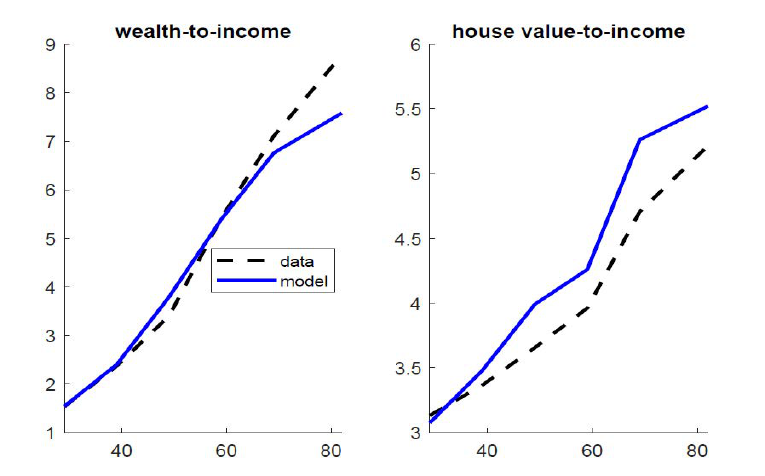
76
!
Figure D1: Model fit of age profiles for household balance sheet positions
This figure plots life-cycle profiles of wealth-to-income and house value-to-income ratios for model versus data. Even though we are
not explicitly targeting life-cycle moments, the model produces a good fit for wealth-to-income ratios and house value-to-income ratios
over the life cycle.
