
Chapter 22:
The CrimeStat Discrete Choice Module
1
Wim Bernasco
NSCR, Amsterdam
&
VU University Amsterdam
Netherlands
Richard Block
Loyola University
Chicago, IL
Ned Levine
Ned Levine & Associates
Houston, TX
Ian Cahill
Cahill Software
Edmonton, AB
The code for the Multinomial Logit and Conditional Logit models was produced by Mr. Ian Cahill of Cahill Software,
Edmonton, Alberta, as part of his MLE++ software package. We have added summary statistics, significance tests, the
routine for creating a conditional logit dataset, and the predictive module. We would like to thank Ms. Haiyan Teng for
her programming.
1
Table of Contents
Discrete Choice Modeling I 22.1
Create Data set for Conditional Discrete Choice Model 22.2
Input Case File 22.4
Case ID 22.5
Choice Variable 22.5
Input Alternatives File 22.5
Alternative ID 22.5
Calculate Distance between Cases and Alternatives 22.5
Save Output 22.6
Estimate Model 22.6
Estimating a Multinomial Logit Model 22.6
Estimating a Conditional Logit Model 22.7
Data File 22.7
Select File for Other Discrete Choice File 22.7
Choice Variable 22.7
Independent Variables 22.7
Type of Discrete Choice Model 22.8
Reference Alternative (multinomial logit model only) 22.8
Case ID (conditional logit model only) 22.9
Output for Discrete Choice Model 22.9
Discrete Choice Model Summary Statistics 22.9
Information about the model 22.9
Discrete choice model likelihood statistics 22.9
Discrete choice individual coefficients statistics 22.10
Average predicted probability 22.11
Multicollinearity Among Independent Variables
in the Discrete Choice Model 22.11
Save Output 22.11
Saved Multinomial Logit Output 22.13
Saved Conditional Logit Output 22.13
Save Estimated Coefficients 22.15
Example of Running a Multinomial Logit Model 22.16
Example of Creating and Running a Conditional Logit Model 22.16
Discrete Choice Modeling II 22.27
Table of Contents
(continued)
Make Prediction 22.27
Discrete Choice Data File 22.27
Discrete Choice Saved Coefficients File 22.27
Available Variables 22.27
Independent Predictors 22.27
Matching Variables 22.27
Alternative values (multinomial logit model only) 22.29
Discrete Choice Data File 22.29
Saved coefficient values (multinomial logit model only) 22.29
Reference alternative (multinomial logit model only) 22.32
Discrete Choice Prediction Output 22.32
Save Predicted Value for Discrete Choice Prediction 22.32
Multinomial Logit Prediction Output 22.32
Conditional Logit Prediction Output 22.33
Chapter 22:
The CrimeStat Discrete Choice Module
We now describe the CrimeStat discrete choice module. There are two pages in the
module. The Discrete Choice I page allows the creation of a data set appropriate for the
conditional logit model and it estimates either multinomial logit or conditional logit models. The
model coefficients can be saved. Using the saved model coefficients, the Discrete Choice II page
calculates predicted probabilities in either the same or another data set.
Discrete Choice Modeling I
The aim of the discrete choice I modeling module is to estimate a functional relationship
between a discrete (nominal) dependent variable and one or more independent variables. It is a
statistical method that is derived from utility theory, i.e. random utility maximization (RUM)
theory. A ‘decision maker’ (e.g., an offender committing a crime) is faced with a set of
alternatives, labeled 1 through J, from which s/he has to select exactly one. The probability that
an alternative will be chosen is a function of its observed and unobserved utility to the decision
maker. The observed utility is a function of known variables and can be expressed as a linear
combination of the independent variables. The unobserved utility is the random error component
of the model. The estimated probability is the exponentiated observed utility of a specific
alternative, J, divided by the sum of the exponentiated observed utilities of all available
alternatives (see Chapter 21).
There are two general forms of the discrete choice model, multinomial logit and
conditional logit. The multinomial logit model estimates the probability that a specific
alternative, 1 to J, as a function of characteristics of the decision makers, either personal
characteristics (e.g., age, gender, ethnicity) or environmental characteristics (e.g., the median
household income of the block in which the decision maker lives). The probability that any one
alternative is chosen is estimated as a function of these characteristics. Per variable
(characteristic), there is one parameter estimated for every alternative, one of which is the
reference alternative in which the coefficients are automatically set to 0. The multinomial logit
model is most appropriate when the outcome of the choice is expected to depend mostly on
characteristics of the decision maker (and not on observed characteristics of the alternatives) and
when there are only a limited number of alternatives available (e.g., 5 weapon choices). The
conditional logit model is a more general model and estimates the probability of a set of
alternatives, 1 to J, as a function of characteristics of the alternatives themselves, possibly in
interaction with characteristics of the decision maker. The conditional logit model is most
appropriate when the outcome of the choice is expected to depend mostly on the characteristics
of the alternatives, and can handle a large number of alternatives. However, the analysis file
22.1
becomes very large. There is a single parameter estimated for every characteristic of the
alternative.
Although the multinomial and the conditional logit are based on a single underlying
statistical model, their estimation requires different data structures. In the multinomial logit
model, the data contain a single record for every decision maker, and a single dependent
(nominal) variable that indicates which alternative (1..J) was chosen. Thus, if there are N
decision makers, there are N records and at least one variable indicates which alternative was
chosen. The file structure is thus similar to that used in the regression module.
In the conditional logit model, for each decision maker there is a record for every choice
that this decision maker is faced. Thus, if there are N decision makers and J alternatives available
to every decision maker, then the data set has N*J records, one for every alternative faced by the
decision maker. In this case, the alternative that was selected has to be indicated by a
dichotomous (dummy) variable (1 for chosen and 0 for not chosen).
Figure 22.1 show the interface for the Discrete Choice I page. The discrete choice I
section includes two routines:
1. A utility for creating a data set appropriate for the conditional logit model. It
matches a data set of Ncases (individuals/offenders/records) with a data set of J
alternatives. The result is a data set with N*J records.
2. A routine for estimating either the multinomial logit model or the conditional logit
model.
Create Data set for Conditional Logit Model
This routine is optional. It simplifies the task of creating a database for use in the
conditional logit model. It matches a case database with a alternatives data base, producing the
cross join of both databases. The case database is the database for the multinomial logit model.
It will thus have the individual records of the decision makers – offenders, individuals,
organizations. It will include at least one variable indicating the alternative that the decision
maker selected (e.g., type of crime committed, the type of weapon used, the location where the
crime was committed) as well as characteristics of the individuals or characteristics associated
with the individuals (e.g., age, gender, ethnicity, median household income of the zone where the
decision maker lives time of event, day of week of event).
The alternatives database, on the other hand, lists the individual alternatives that were
available (e.g., all the locations where a crime could be committed, all the different types of
22.2

Figure 22.1:
Discrete Choice Modeling I
weapons that were used by different offenders) as well as attributes associated with the
alternatives themselves (e.g., median household income or number of employees working at the
locations, or characteristics associated with each type of weapon).
The joined file has one record per alternative for each case. Thus, if there are N
individuals faced with J choices, then the matching routine will create N*J records. It should be
noted that the matching assigns every characteristic associated with a choice to every case
associated with a decision maker. A field, called CHOSEN, is automatically added to every
record. This field has the value 1 for alternatives that were chosen and 0 for alternatives that
were not chosen. The Chosen field should thus sum to N (i.e., only one record per decision
maker should have a selected alternative). Also, as an option, and only if both the individuals
and the alternatives have geographic coordinates, a second field called DISTANCE will be added
that calculates the distance from each case record to each alternative record. The user must
specify which distance units are to be used (miles, kilometers, meters, feet, or nautical miles).
For example, if both the case database and the alternatives database contain X and Y
coordinates, then it is possible to calculate the distance between every decision maker and every
choice.
The routine cannot calculate other interactions associated with a specific alternative and
particular decision maker, and such interactions must be added to the data outside CrimeStat.
Interactions between variables in the data can be calculated. For example, to test whether
increasing distance makes alternatives less attractive for juvenile offenders but not for adult
offenders, an interaction DISTANCE x AGE can be calculated. Other interactions require
additional information, for example if location choice is what is modeled, one may want to add a
variable indicating, for each alternative location, how many prior offences the offender has
committed in that alternative location. In these cases the external file is constructed by the user,
and the step “Create data set for conditional discrete choice model” is skipped.
Input Case File
The case data set for the Discrete Choice I module can be the Primary file, the Secondary
file, or another file. If the Primary file or Secondary files are used, the coordinate system and
distance units were defined on the Primary file page. If another file is used, then any coordinates
in that file are not defined and the file is treated as a non-spatial file. The user must browse and
identify the file. To avoid confusion, the user must verify that no variable/field in the input case
file has the same name as any variable in the Input Alternatives File (see below). Note: If a
primary file is used, coordinates must be defined for that file. If the file is not spatial, then input
it as ‘Other file’.
22.4
Case ID
Select the Case ID. The Input Case File must have a Case ID, a variable that uniquely
identifies cases in the Input Case File.
Choice Variable
Select the Choice Variable. The Input Case File must contain a variable (field) that
identifies alternative chosen by the decision maker. For example, if the choice is about the type
of weapon used, then the Choice Variable indicates whether it was a gun, a knife , strong-arm,
and so forth. Or, if the choice is the census tract in which a crime was perpetrated, then the
Choice Variable identifies the census tract where the incident occurred.
Input Alternatives File
The alternatives data set for the Discrete Choice I module can be the Primary file, the
Secondary file, or another file. If the Primary or Secondary files are used, the coordinate system
and distance units were defined on the Primary file page. If another file is used, then any
coordinates in that file are not defined and the file is treated as a non-spatial file. The user must
browse and identify the Input Alternatives File. To avoid confusion, the user must verify that no
variable in the input alternative file has the same name as any variable in the Input Case File.
Alternatives ID
Select the Alternatives ID. The Alternatives File must have an Alternative ID, a variable
that uniquely identifies records in file. The Alternatives File must contain a record for every
possible alternative even those that were never chosen. For example, most census tracts in a city
have no homicides during a year, but the alternatives file must include every tract. The coding
must match the coding of the Choice Variable in the Input Case File. Be careful about duplicate
ID names in the two files as the name will appear twice in the output file with the first use
representing the cases and the second use representing the alternatives. The names reflect the
link between each case ID and each alternatives ID and it is better to use different names for the
ID fields to avoid confusion.
Calculate Distance between Cases and Alternatives
There is an optional box that allows the routine to calculate the distance from each case
record to each alternative record. If checked, the routine will calculate the distance. This only
applies if both the case file and the alternatives file are either the Primary file or Secondary. The
user must specify the distance units to be used in the calculation (in miles, kilometers, feet,
22.5
meters, or nautical miles). The box is checked by default. The saved filed will have a new field
called DIST. That is, if the X/Y coordinates for an offender’s home address are coded in the
Input Case File while the coordinates for census tract are recorded in the Input Alternatives File,
then the distances from the offender’s home to each alternative census tract will be calculated.
Save Output
The matched Input Case and Input Alternatives file is saved as a new file in ‘dbf’ format,
that can subsequently be used to estimate a conditional (but not multinomial) logit model, as
described below under ‘Estimating a conditional logit model’. The user should define the name
of the file and point to the directory where it is saved. The output includes all fields from the
case file and all fields from the choice file, and optionally a field DIST containing calculated
distances. There will be J records for each of the N cases. An automatically added field called
CHOSEN takes the value ‘1’ for the choice that was selected and ‘0’ for choices that were not
selected.
Note that the joined data base can be very large. Before creating a data set for a
conditional discrete choice model, include in the alternatives and choice files only variables that
are likely to be used in the analysis, and to format them to be as small as possible.
Estimate Model
The Estimate Model routine will estimate a discrete choice model, either the multinomial
logit or the conditional logit.
Estimating a Multinomial Logit Model
The multinomial logit model is used when there is one record per decision maker with a
choice having been made by the decision maker. The model estimates the effect of each
independent variable on the probability of each distinct alternative. The data are structured so
that there is one record per decision maker with the choice variable indicating which alternative
was chosen. The data set is similar to that of the regression model in that there is one record per
decision maker. The model then estimates the effects of the independent variables on the
probability of each alternative. By definition, one of the alternatives (by default the most
frequently chosen alternative, otherwise to be chosen by the user) is the reference alternative to
which the other alternatives are compared.
The multinomial logit model is always estimated with a constant. This type of model is
appropriate when values of the predictor variables only vary across cases (decision-makers), not
across alternatives.
22.6
Estimating a Conditional Logit Model
The conditional logit model, on the other hand, is used when the values of the predictor
variables vary across alternatives. In that case, there is one record per alternative per decision
maker. That is, the decision maker is faced with J alternatives but chooses only one. The
database must indicate which of the J alternatives was selected and the model estimates the
effect of each independent variable on choosing an alternative. There is a record for every
alternative faced by the decision maker. The parameter estimates indicate the effects of the
independent variables on the likelihood that the alternative is selected.
Data File
The data set for the model can be either the Primary file or another file (the Secondary
file is not available). If the Primary file is used, the coordinate system and distance units are the
same as were defined on the Primary file page.
Select file for Other Discrete Choice File
If the discrete choice file is another file than the Primary file, the user must browse and
identify the file.
Choice Variable
A list of variables from the discrete choice file is displayed. There is a box for defining
the choice variable. The user must select one choice variable. . For the conditional logit model,
on the other hand, the variable contains a set of 1’s (for selected alternatives) or 0’s (for
alternatives that were not selected). If the data set was constructed with the CrimeStat ‘Create
data set for conditional discrete choice model’ routine, then the field CHOSEN should be used.
Note that the field that is added for the choice variable (whether CHOSEN or another
variable) is inspected for unique values. If the data set is large, it may take a while to filter
through those values.
Independent Variables
There is a box for defining the independent variables. The user must choose one or more
independent variables. There is no limit to the number. The variables are output in the same
order as specified in the dialogue so a user should consider how these are to be displayed. The
order in which the variables are entered does not affect the estimated parameters.
22.7
Type of Discrete Choice Model
The type of discrete choice model to be estimated must be specified. The choices are
Multinomial (logit) or Conditional (logit). The default model is the Conditional logit. NOTE: the
file used for a Multinomial Logit model is different than the file used for a Conditional Logit
model. With the file used in the Multinomial Logit model, there is one record per case with the
choice specified on the record. With the file used in the Conditional Logit model, there is one
record per alternative with J records per case (where J is the number of alternatives). Be sure to
use the correct file type. The routine assumes that the data are consistent with the type of model
chosen. For a multinomial logit model, the routine will treat each record as a separate decision
maker and will estimate a model for each choice less the reference choice. For a conditional
logit model, the routine will treat each record as one of J choices (where J is defined by the user
– see below) and will estimate a single model for the decision.
The user needs to be very careful that the correct data set is used with the appropriate
model because the routine can estimate its equations with either of these data sets. That is, if the
data set is appropriate for the multinomial logit model but the user specifies a conditional logit
model, the routine will estimate a single equation treating multiples of J records as a single
decision maker. Similarly, if the data set is appropriate for a conditional logit model but the user
specifies a multinomial logit model, the routine will treat each record as if it were a separate
decision maker and will estimate one equation for each choice that it finds in the choice variable.
The results in both these cases will be meaningless since the there is a mismatch between the
data set and the type of model selected. In short, the user should be aware of this.
Reference Alternative (multinomial logit model only)
For the multinomial logit model, the user should specify which choice is to be used as the
reference. The constant and the coefficients for the reference choice will automatically be 0. The
user should specify a particular choice from the list of available alternatives or select the most
frequently used alternative as the reference choice. Keep in mind that the coefficients will
change depending on which alternative is selected as the reference choice since a comparison is
always relative. This will affect the interpretation of the coefficients though not the estimated
probabilities.
For the conditional logit model, however, there is no reference choice. Therefore, this
field will be blanked out when the type of discrete choice model is conditional.
22.8
Case ID (conditional logit model only)
When a conditional logit model is estimated, each case contributes multiple records to the
data file (as many as there are alternatives). In order for CrimeStat to know which records belong
to the same case (decision maker), the user must specify a Case ID variable, i.e. a variable that
uniquely identifies cases (decision makers). If the data set was created with the CrimeStat
‘Create Data set for Conditional Logit Model’ routine, the variable is the Case ID variable
specified in that routine. CrimeStat will check the number of alternatives per case, and only
estimate the conditional logit model if all cases have an equal number of alternatives. If the
number of alternatives per case is not equal, CrimeStat will issue an error message upon the start
of the estimation.
Output for the Discrete Choice Model
The output includes both summary statistics and individual variable coefficients
estimates. The output will vary between the multinomial logit and conditional logit models.
Discrete Choice Model Summary Statistics
The summary statistics include:
Information about the model
1. Date and time
2. The data file
3. The dependent (choice) variable
4. The number of records
5. The degrees of freedom
6. The type of choice model (multinomial discrete or conditional discrete)
7. Number of alternatives. For both the multinomial logit model and the conditional
logit model, the routine will internally determine the number of alternatives.
8. The method of estimation (MLE – maximum likelihood estimation)
Discrete choice model likelihood statistics
9. Log likelihood estimate, which is a negative number. For a set number of
independent variables, the smaller the log likelihood (i.e., the most negative) the
better.
10. Log likelihood per case. Smaller (more negative) values are better. This is useful
when comparing a similar model but with different numbers of records.
22.9
11. Akaike Information Criterion (AIC) adjusts the log likelihood for the degrees of
freedom. The smaller the AIC, the better.
12. AIC per case. Smaller values are better.
13. Bayesian Information Criterion (BIC), sometimes known as the Schwartz
Criterion (SC), adjusts the log likelihood for the degrees of freedom. The smaller
the BIC, the better.
14. BIC per case. Smaller values are better.
15. Mean Absolute Deviation (MAD). For a set number of independent variables, a
smaller MAD is better.
16. Mean Squared Predictive Error (MSPE). For a set number of independent
variables, a smaller MSPE is better.
Discrete Choice Individual Coefficients Statistics
There is different coefficient output for the multinomial logit model than for the
conditional logit model. The multinomial logit model will output constants and individual
coefficients for each of J-1 alternatives (where J is the total number of alternatives). The constant
and coefficients for the reference alternative are automatically defined as zero (0). For example,
if there are four alternatives, then three sets of equations will be output, one for each of the J-1
(4-1=3) alternatives. The coefficients are always relative to the reference alternative. Therefore,
a positive coefficient indicates that the independent variable contributes more for that alternative
than for the reference alternative while a negative coefficient indicates that the independent
variable contributes less for that choice than for the reference choice. The significance test of the
coefficient indicates whether the difference is statistically significant or not compared to the
reference alternative. Note that the multinomial logit model always has a constant.
On the other hand, the conditional logit model will output a single set of individual
coefficients with no constant. There is no reference choice and the coefficients are relative to
not choosing a particular alternative (i.e., having a value of 0 for CHOSEN).
For the individual coefficients, the following are output for each independent variable:
1. The coefficient.
2. The standard error of the coefficient.
3. t-value.
4. p-value. This is the two-tail probability level associated with the t-test.
5. Odds ratio. This is the exponentiation of the coefficient (i.e., e
β
). It indicates the
change in the odds of that alternative (relative to the reference alternative in the
multinomial model, and relative to 0 in the conditional logit model) caused by a
one-unit increase in the independent variable.
22.10
Average predicted probability
For the conditional logit model only, an additional table is output that indicates the
average predicted probability of the model for those cases that were selected (i.e., in which
CHOSEN=1), for those cases that were not selected (i.e., CHOSEN=0), and for all cases. The
number of records associated with each category is indicated as well as the standard deviation.
Table 22.1 show the output for two of the weapon alternatives for a multinomial logit
model predicting weapon use during 2006 Houston robberies. Only the first two weapon
alternatives (bodily force and firearms) are shown.
Multicollinearity Among Independent Variables in the Discrete Choice Model
A major consideration in any regression model (including discrete choice) is that the
independent variables are statistically independent. Non-independence is called multicollinearity
and means that there is overlap in prediction among two or more independent variables. This
can lead to uncertainty in interpreting coefficients as well as to an unstable model that may not
hold in the future. Generally, it is a good idea to reduce multicollinearity as much as possible.
A tolerance test is given for each coefficient. This is defined as 1 – the R-square of the
independent variable predicted by the remaining independent variables in the equation using an
Ordinary Least Squares model. It is an indicator of how much the remaining variables in a
model account for the variance of any particular independent variable. Since the method uses the
Ordinary Least Squares (OLS) methods, it is an approximate (pseudo) test for the discrete choice
routines. OLS assumes normality and constant residual errors. However, many independent
variables are not normally distributed (e.g., income, distance traveled, number of persons living
in poverty). Consequently, the use of OLS to test for multicollinearity is exact only when the
independent variable being examined for tolerance is normally distributed; otherwise, it is an
approximate test. Nevertheless, it is useful indicator of multicollinearity. If the tolerance is low,
that definitely indicates that there is multicollinearity. On the other hand, a high tolerance level
does not necessarily indicate that there is little multicollinearity.
From the test, a guidance message is displayed that indicates probable or possible
multicollinearity. If there is substantial multicollinearity (indicated by low tolerance values), it is
a good idea is to drop one of the colinear independent variables and re-run the model.
Save Output
The output from the discrete choice model can be saved.
22.11
-----------------------------------------------------------------------------
-----------------------------------------------------------------------------
-----------------------------------------------------------------------------
Model result:
Data file: Houston robberies 2007-2009.dbf
DepVar: WEAPON
N: 3709
Df: 3697
Type of choice model: Multinomial logit model
Number of Alternatives: 5
Method of estimation: MLE
Likelihood statistics
Log Likelihood: -4432.143485
Per case: -1.194970
AIC: 8936.286971
Per case: 2.409352
BIC/SC: 9160.153603
Per case: 2.469710
Model error estimates
Mean absolute deviation: 0.319935
Mean squared predicted error: 0.184770
Predictor
-------------
Coefficient
--------------
Stand Error
--------------
t-value
------------
p-value
-----------
Odds Ratio
-------------
Bodily force
Alternative N=1184
Constant 0.538440 0.005424 99.266258 0.001 1.713332
PRIMAGE -0.001171 0.002809 -0.416833 n.s. 0.998830
PRIMGENDER 0.054200 0.005423 9.994519 0.001 1.055695
HISPANIC 0.236188 0.005416 43.606294 0.001 1.266412
BLACK 0.580160 0.005414 107.168407 0.001 1.786324
NUMSUSPCTS -0.134192 0.005376 -24.959032 0.001 0.874422
COMMERCIAL 0.296323 0.005417 54.700174 0.001 1.344904
NIGHT 0.086105 0.005421 15.884819 0.001 1.089921
AFTERNOON 0.463824 0.005416 85.641166 0.001 1.590144
MORNING 0.338060 0.005422 62.350883 0.001 1.402224
CL_MDHHINC 0.000011 0.000003 4.135364 0.001 1.000011
DISTANCE -0.022691 0.004519 -5.021083 0.001 0.977565
Firearm
Alternative N=1744
Constant 0.495888 0.005424 91.425683 0.001 1.641956
PRIMAGE -0.027863 0.002846 -9.791397 0.001 0.972521
PRIMGENDER -0.930784 0.005424 -171.601872 0.001 0.394245
HISPANIC 1.031718 0.005415 190.544383 0.001 2.805882
BLACK 1.397967 0.005412 258.286949 0.001 4.046965
NUMSUSPCTS 0.177425 0.005363 33.080392 0.001 1.194139
COMMERCIAL 0.643070 0.005416 118.730846 0.001 1.902312
NIGHT 0.392673 0.005418 72.470517 0.001 1.480934
AFTERNOON -0.211853 0.005416 -39.114246 0.001 0.809084
MORNING 0.167169 0.005421 30.835798 0.001 1.181955
CL_MDHHINC 0.000005 0.000003 1.970048 0.050 1.000005
DISTANCE 0.028941 0.004351 6.652022 0.001 1.029364
Table 22.1
Multinomial Logit Model Screen Output
22.12
Saved Multinomial Logit Output
For the multinomial logit model, the output is a ‘dbf’ file that includes all the input
variables along with the estimated probability for each choice and the residual error for each
choice (the observed choice, 1 or 0, minus the predicted probability). The probability and
residual error is presented for each of the J alternatives. These are labeled with a ‘P_ ‘ for
probability and ‘R_’ for residual error. The different alternatives are indicated by a subscript
from 0 (for the reference choice) through J-1 (for the other alternatives) in the same order in
which they are listed in Reference Choice dialogue (excluding the reference choice itself). For
example, P_Choice0 is the estimated probability for choice 0 (the reference choice) while
R_Choice3 is the estimated residual error for choice 3 (the third one listed in the list under
Reference Choice excluding the reference choice itself). Table 22.2 shows the first 25 records of
the file output from the Multinomial Logit model.
Saved Conditional Logit Output
For the conditional logit model, the output is a ‘dbf’ file and includes all the input
variables along with the estimated probability and the residual error for the case. For each case
ID, there will be only one record that was chosen. Further, since the conditional logit model
produces only one equation, there is only one probability and one residual error. The probability
is labeled PREDPROB and the residual error is labeled RESID. The residual error can be used
to compare different models. The MAD and MSPE statistics (discussed above) summarize the
residual errors. But, a user might want to plot the residuals against one of the independent
variables to see if it the errors are continuous and increasing (well behaved). A bizarre error
pattern can usually indicate that an independent variable is not appropriate.
Specify a directory where the output file is to be saved and provide a root name. The
saved file for the multinomial logit model will have a DCOutMNL prefix while the saved file for
the conditional logit model will have a DCOutCNL prefix before the user defined root name.
Table 22.3 shows the first 32 records from the file output for the conditional logit model
that was set up in Figure 22.9 the output of which is display in Figure 22.11. This file copies the
input records and adds the predicted probability (PREDPROB) for each case-alternative
combination. For example, for Case 1 the probability of choosing TAZ 403 equals 0.000370.
Note that within these first 32 zones, the probability of Case 1 choosing TAZ 429 is highest
(0.046303),which happens to be the TAZ actually chosen by the offender (CHOSEN=1).
22.13
Make prediction:
---------------------------------------------------------
Data file: Houston robberies 2010.dbf
Type of discrete choice model: Multinomial discrete model
N: 3709
Predicted Probabilities
--------------------------
Case ID Choice0 Choice1 Choice2 Choice3 Choice4
1 0.056060 0.370066 0.331705 0.073570 0.168599
2 0.096763 0.431871 0.365920 0.060182 0.045264
3 0.082294 0.316838 0.508919 0.049205 0.042744
4 0.183496 0.380540 0.208544 0.152571 0.074849
5 0.092852 0.248848 0.570410 0.045357 0.042533
6 0.054154 0.410175 0.446969 0.036294 0.052408
7 0.043498 0.405445 0.451540 0.029337 0.070181
8 0.083722 0.252532 0.522326 0.118092 0.023329
9 0.082219 0.156078 0.665132 0.077454 0.019117
10 0.080632 0.448033 0.371738 0.048678 0.050919
11 0.086503 0.273349 0.552494 0.045244 0.042410
12 0.144867 0.576979 0.041781 0.187909 0.048464
13 0.048195 0.159970 0.734329 0.020854 0.036652
14 0.107029 0.195817 0.633713 0.044797 0.018644
15 0.115121 0.322193 0.338518 0.168298 0.055870
16 0.090629 0.491720 0.283552 0.071254 0.062845
17 0.078795 0.591412 0.262103 0.042796 0.024894
18 0.122961 0.270860 0.446626 0.127957 0.031596
19 0.074225 0.261177 0.516627 0.094802 0.053169
20 0.156918 0.364621 0.132714 0.280764 0.064982
21 0.052718 0.322463 0.475312 0.032347
0.117159
22 0.081029 0.416482 0.297664 0.133562 0.071264
23 0.114424 0.425378 0.377130 0.070873 0.012195
24 0.081482 0.400866 0.316524 0.126742 0.074385
25 0.185771 0.322145 0.298299 0.111579 0.082205
Table 22.2:
File Output from Multinom
ial Logit Model
First 25 Records
22.14
CASE TAZ AREA ARTERIAL COMMACRES DIST_CBD DISTANCE CHOSEN PREDPROB
1 401 35.97 0.00 14.01 28.01 29.95 0 0.000000
1 402 37.64 13.65 54.58 26.96 34.87 0 0.000000
1 403 8.23 6.66 66.95 21.63 23.04 0 0.000370
1 404 11.10 2.96 0.00 22.42 24.90 0 0.000042
1 405 25.22 12.91 11.08 24.43 26.95 0 0.000001
1 406 21.48 10.70 7.26 20.73 21.92 0 0.000003
1 407 9.40 9.95 54.11 20.18 19.40 0 0.000410
1 408 10.26 0.65 0.00 19.31 18.52 0 0.000091
1 409 4.87 2.48 0.00 16.97 15.38 0 0.000795
1 410 5.49 0.38 0.00 18.28 17.80 0 0.000441
1 411 3.23 0.00 0.00 17.03 16.16 0 0.001030
1 412 4.43 2.38 2.57 19.28 20.98 0 0.000511
1 413 2.56 2.78 2.90 16.80 18.97 0 0.001039
1 414 3.03 1.52 1.66 16.09 18.66 0 0.000781
1 415
7.62 0.00 0.00 18.23 18.97 0 0.000175
1 416 4.13 1.98 0.00 17.05 15.44 0 0.000983
1 417 5.01 0.82 0.00 16.47 15.23 0 0.000655
1 418 8.85 4.72 1.36 22.32 27.84 0 0.000065
1 419 11.00 3.07 8.28 19.66 24.66 0 0.000038
1 420 11.93 2.51 0.36 17.48 18.81 0 0.000047
1 421 4.68 5.87 20.41 14.96 17.75 0 0.000773
1 422 4.41 2.87 15.36 17.13 23.06 0 0.000360
1 423 3.27 0.22 0.00 15.49 21.08 0 0.000420
1 424 5.27 0.36 28.30 14.03 16.51 0 0.000512
1 425 0.88 0.00 62.12 14.35 10.67 0 0.007878
1 426 0.52 0.00 10.82 13.45 10.26 0 0.004882
1 427 0.37 0.00 0.00 12.84 9.46 0 0.004833
1 428 0.80 0.00 0.00 13.56 10.26 0 0.003989
1
42
9 0.40 0.00 201.95 12.76 9.23 1 0.046303
1 430 3.83 0.00 21.03 15.02 12.46 0 0.001520
1 431 0.23 0.67 19.12 14.70 12.15 0 0.005282
1 432 0.70 0.00 0.00 14.79 11.92 0 0.003635
Table 22.3:
File Output from Conditional Logit Model
First 32 records
Save Estimated Coefficients
The coefficients from either the multinomial logit or the conditional logit models can be
saved for use with other data sets. Specify a directory where the coefficients file is to be saved
and provide a root name. The saved coefficients file for the multinomial logit model will have a
DCCoeffMNL prefix while the saved coefficients file for the conditional logit model will have a
DCCoeffCNL prefix before the user defined root name.
22.15
Example of Running a Multinomial Logit Model
To illustrate the process of running a multinomial logit model, we model the premises
chosen for Chicago residential robberies for 1997. Figure 22.2 shows setting up the multinomial
logit model including reading in the data file as the ‘Other’ file, defining the choice variable
(PREMISES) and the selection of the predictors from the list of available independent variables
(GUNCRIME, EVENING, LATENIGHT, TRAVELDIST, OFFAGE, and OFFBLACK).
Finally, Figure 22.3 shows the screen output of the multinomial logit model.
Example of Creating and Running a Conditional Logit Model
To illustrate the process of creating a file for the conditional logit model and then running
a file to estimate the predictors of the alternatives, we use an example of predicting which Traffic
Analysis Zone (TAZ) offenders use to commit crimes. In Figure 22.4, the case file, which
contains the origin TAZ and destination TAZ of each of 500 offences, is input as the Primary
File and the coordinates of each crime location are input as the X and Y coordinates.
In Figure 22.5, the alternatives file is the information on the 325 TAZs themselves. This
is input on the Secondary File page and the coordinate for each TAZ are defined. In figure 22.6,
both the case file and the alternatives file are defined for the ‘Create data set for conditional logit
model’ routine. The case file is defined by the Primary File with the case ID being CASE. The
alternatives file (the TAZs) are defined by the secondary File with the alternative ID being TAZ.
The ‘Calculate distance between cases and alternatives’ box is checked and the distance units
will be calculated in miles.
Figure 22.7, the file for the created file is defined (CasesXAlternatives.dbf). Once the
user calculates ‘Compute’, the routine runs. When it has finished, it gives a ‘File saved’ message
(Figure 22.8).
The user should be sure to uncheck the ‘Create data set for conditional logit model’
routine box. Then, either the created file or another file prepared by the user is input as the
Primary File. On the Discrete Choice I page, the ‘Estimate Model’ box is checked and the
conditional logit model is set up. The dependent variable is CHOSEN if the file was created by
the cross-joined file, and can have any name if it was prepared by the user. The dependent
variable must be a binary (0/1) variable. Subsequently, several appropriate predictor variables
are selected from the independent variables list (Figure 22.9). In the Conditional Logit example
they are AREA, ARTERIAL, COMMACRES, DIST_CBD and DISTANCE An output file is
then defined to save the results of the conditional logit model (Figure 22.10). Once the
conditional logit model is run, the screen output can be viewed (Figure 22.11).
22.16

Figure 22.2:
Example of Running a Multinomial Logit Model
Step 1 Setting Up the Multinomial
Logit
Model
Step 1
:
Setting Up the Multinomial
Logit
Model

Figure 22.3:
Example of Running a Multinomial Logit Model
Step 2 Results of the Multinomial
Logit
Model Estimate
Step 2
:
Results of the Multinomial
Logit
Model Estimate

Figure 22.4:
Example of Setting Up and Running a Conditional Logit Model
Step 1 Inputting a Case File as the Primary File
Step 1
:
Inputting a Case File as the Primary File

Figure 22.5:
Example of Setting Up and Running a Conditional Logit Model
Step 2 Inputting an Alternatives File as the Secondary File
Step 2
:
Inputting an Alternatives File as the Secondary File

Figure 22.6:
Example of Setting Up and Running a Conditional Logit Model
Step 3 Setting Up the Routine for Creating a Conditional
Logit
Database
Step 3
:
Setting Up the Routine for Creating a Conditional
Logit
Database
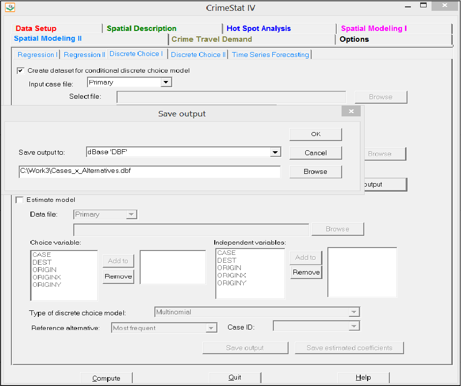
Figure 22.7:
Example of Setting Up and Running a Conditional Logit Model
Step 4 Choosing a File Name to Save the Created File
Step 4
:
Choosing a File Name to Save the Created File

Figure 22.8:
Example of Setting Up and Running a Conditional Logit Model
Step 5 Running the Routine to Create the File
Step 5
:
Running the Routine to Create the File

Figure 22.9:
Example of Setting Up and Running a Conditional Logit Model
Step 6 Setting Up Conditional
Logit
Model
Step 6
:
Setting Up Conditional
Logit
Model
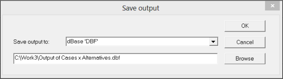
Figure 22.10:
Example of Setting Up and Running a Conditional Logit Model
Step 7 Defining Output File for the Conditional
Logit
Model
Step 7
:
Defining Output File for the Conditional
Logit
Model

Figure 22.11:
Example of Setting Up and Running a Conditional Logit Model
Step 8 Screen Output for the Conditional
Logit
Model
Step 8
:
Screen Output for the Conditional
Logit
Model
Discrete Choice Modeling II
The Discrete Choice modeling II module allows the user to apply the estimated
coefficients from a discrete choice model to another data set (or a subset of the same data set)
and calculate predicted probabilities, for either the multinomial logit or the conditional logit
model. The ‘Make prediction’ routine allows the application of coefficients to a data set. The
saved coefficients are applied to similar independent variables and to corresponding values of the
choice variable to produce an estimated probability of an alternative.
Make Prediction
Figure 22.12 show the interface for the Discrete Choice II page. There are two types of
models that can be fitted – multinomial logit or conditional logit. For both types of model, the
coefficients file must include information on each of the coefficients. In addition, the
coefficients model for the multinomial must include the value of the constant. If the coefficients
file was generated by CrimeStat on the Discrete Choice I page, then all the necessary information
will be included. The user reads in the saved coefficient file and matches the variables to those
in the new data set based on the order of the coefficients file.
Discrete Choice Saved Coefficients File
In order to make a prediction, a model must have already been calibrated and the
coefficients saved in a coefficients file. Point to the directory where the coefficients file has
been saved and identify it.
Available Variables
The box labeled ‘Available variables’ will list all the fields on the input data set.
Independent Predictors
The independent variables that were used in the calibrated coefficients file will be listed
in the right column. They will be in the same order as was estimated in the calibration file.
Matching variables
Select corresponding variables from the input data file for the middle column. The items
should be listed in the same order as in the ‘independent predictors’ column. They should be
22.27

Figure 22.12:
Discrete Choice Modeling II
similar variables in content but need not have the names as in the original data file. Figure 22.13
shows an example of setting up a multinomial logit prediction model using an already estimated
multinomial logit model from another data set. The user reads in the data file and then already-
saved coefficients from the earlier calibration and then matches the variable names in the new
data set with the saved names from the already calibrated model. In the example, the variable
names for travel distance were different in the two files.
Figure 22.14 shows an analogous example of setting up a conditional logit prediction.
Again, the variable names in the input file on which the prediction is to be calculated (AREA,
ARTERIAL, etc.), are the same as those in the file on which the coefficients were estimated.
This also holds for the ID variable name, which must be specified in case of a conditional logit
prediction.
Alternative values (multinomial logit model only)
The values of the choice variables from the input file will be displayed in the middle
column. The order should match the values in the adjacent saved coefficients file column. The
‘Up’ and ‘Down’ buttons can be used to re-order the values to be sure they are matched exactly.
Discrete Choice Data File
The new data set can be either the Primary file or another file. If another file is being
used, point to the directory where it is stored and identify it. The structure of the file for which a
prediction is made must be the same as that from which the model was initially calibrated. That
is, for a multinomial logit prediction, there must be a file with one record per decision maker and
which includes and ID and each of the independent variables used in the prediction. For a
conditional logit prediction, there must be a joined file with a record for every combination of
case and alternative.
Saved coefficient values (multinomial logit model only)
The values of the saved coefficients file will be displayed in the right column. Additional
values can be added with the “Add to” button and existing values can be removed with the
“Remove” button. It is essential that the values in the middle column match exactly their
corresponding values in the right column.
22.29

Figure 22.13:
Example of Running a Multinomial Logit Prediction

Figure 22.14:
Example of Running a Conditional Logit Prediction
Reference alternative (multinomial logit model only)
The reference alternative value is displayed. If it is not correct, type in the correct value
to be used or, better yet, re-calibrate the original model. This field will be blanked out for the
conditional logit model since it is not appropriate.
Discrete Choice Prediction Output
The screen output provides predictions of the value of the dependent variable in the same
order as in the input data set. For the multinomial logit model, the predictions are labeled as
CHOICE0 (for the reference choice), CHOICE1, CHOICE2, and so forth, in the same order as in
the input data set. For each alternative, these predictions represent the probability that this
alternative is chosen, given the values of the predictor variables.
For the conditional logit model, the prediction is applied to each available alternative.
The screen output presents the predictions in matrix format with the case ID listed on the vertical
axis and the choices listed on the horizontal axis (labeled CHOICE0, CHOICE1, CHOICE2, and
so forth, in the same order as in the input data set).
Save Predicted Values for Discrete Choice Prediction
The predicted values and the residual errors can be output to a ‘dbf’ file with a
DCMakePredMNL<root name> for the multinomial logit and DCMakePredCNL<root name>
for the conditional logit with the root name being provided by the user. The output files differ
between the multinomial and conditional logit models.
Multinomial Logit Prediction Output
For the multinomial logit prediction, there is the probability produced for each of the J
alternatives. The probabilities are labeled P_CHOICE0 (for the reference choice), P_CHOICE1,
P_CHOICE2, and so forth in the same order as in the Choice Values dialogue (with the
exception of the reference alternative which is always defined as P_CHOICE0). The
probabilities will sum to 1.0 for all J alternatives (within rounding-off error).
Table 22.4 shows the first 25 cases for the file output of a multinomial logit prediction of
weapon use for 2010 Houston robberies. The specific alternatives are labeled Choice0, Choice1,
Choice2, Choice3, and Choice4 and are the weapon categories in the same order as laid out on
the interface (namely Other weapon, Bodily force, Firearm, Knife, and Threat).
22.32
ID P_CHOICE0 P_CHOICE1 P_CHOICE2 P_CHOICE3 P_CHOICE4
1 0.056060 0.370066 0.331705 0.073570 0.168599
2 0.096763 0.431871 0.365920 0.060182 0.045264
3 0.082294 0.316838 0.508919 0.049205 0.042744
4 0.183496 0.380540 0.208544 0.152571 0.074849
5 0.092852 0.248848 0.570410 0.045357 0.042533
6 0.054154 0.410175 0.446969 0.036294 0.052408
7 0.043498 0.405445 0.451540 0.029337 0.070181
8 0.083722 0.252532 0.522326 0.118092 0.023329
9 0.082219 0.156078 0.665132 0.077454 0.019117
10 0.080632 0.448033 0.371738 0.048678 0.050919
11 0.086503 0.273349 0.552494 0.045244 0.042410
12 0.144867 0.576979 0.041781 0.187909 0.048464
13 0.048195 0.159970 0.734329 0.020854 0.036652
14 0.107029 0.195817 0.633713 0.044797 0.018644
15 0.115121 0.322193 0.338518 0.168298 0.055870
16 0.090629 0.491720 0.283552 0.071254 0.062845
17 0.078795 0.591412 0.262103 0.042796 0.024894
18 0.122961 0.270860 0.446626 0.127957 0.031596
19 0.074225 0.261177 0.516627 0.094802 0.053169
20 0.156918 0.364621 0.132714 0.280764 0.064982
21 0.052718 0.322463 0.475312 0.032347
0.117159
22 0.081029 0.416482 0.297664 0.133562 0.071264
23 0.114424 0.425378 0.377130 0.070873 0.012195
24 0.081482 0.400866 0.316524 0.126742 0.074385
25 0.185771 0.322145 0.298299 0.111579 0.082205
Table 22.4:
File Output from Multinomial Logit Prediction Routine
First 25 records
Conditional Logit Prediction Output
For the cond
itional logit prediction, there is a single probability output which is applied
to the particular record. Since the data set for the conditional logit model has a single record for
each alternative available to the decision maker, the probability applies to that alternative. The
probabilities within a case will sum to 1.0 for all J alternatives (within rounding-off error). The
column is labeled PREDPROB. Table 22.5 shows the first 32 cases for a CL prediction output.
22.33
CASE TAZ AREA ARTERIAL COMMACRES DIST_CBD DISTANCE PREDPROB
501 401 35.97 0.00 14.01 28.01 31.59 0.000000
501 402 37.64 13.65 54.58 26.96 34.76 0.000000
501 403 8.23 6.66 66.95 21.63 23.78 0.000331
501 404 11.10 2.96 0.00 22.42 26.45 0.000033
501 405 25.22 12.91 11.08 24.43 30.25 0.000000
501 406 21.48 10.70 7.26 20.73 25.48 0.000002
501 407 9.40 9.95 54.11 20.18 25.72 0.000158
501 408 10.26 0.65 0.00 19.31 24.38 0.000037
501 409 4.87 2.48 0.00 16.97 20.48 0.000368
501 410 5.49 0.38 0.00 18.28 25.22 0.000144
501 411 3.23 0.00 0.00 17.03 23.86 0.000322
501 412 4.43 2.38 2.57 19.28 21.17 0.000496
501 413 2.56 2.78 2.90 16.80 19.37 0.000979
501 414 3.03 1.52 1.66 16.09 18.08 0.000852
501 415 7.62 0.00 0.00 18.23 20.75 0.000134
501 416 4.13
1.98 0.00 17.05 18.92 0.000580
501 417 5.01 0.82 0.00 16.47 17.45 0.000469
501 418 8.85 4.72 1.36 22.32 26.56 0.000080
501 419 11.00 3.07 8.28 19.66 21.68 0.000059
501 420 11.93 2.51 0.36 17.48 16.77 0.000064
501 421 4.68 5.87 20.41 14.96 14.64 0.001236
501 422 4.41 2.87 15.36 17.13 19.13 0.000653
501 423 3.27 0.22 0.00 15.49 16.58 0.000830
501 424 5.27 0.36 28.30 14.03 12.03 0.001008
501 425 0.88 0.00 62.12 14.35 17.89 0.002650
501 426 0.52 0.00 10.82 13.45 17.67 0.001596
501 427 0.37 0.00 0.00 12.84 16.84 0.001586
501 428 0.80 0.00 0.00 13.56 18.02 0.001236
501 429 0.40 0.00 201.95 12.76 16.85 0.014658
501 430 3.83 0.00 21.03 15.02 20.21 0.000472
501 431 0.23 0.67 19.12 14.70 19.10 0.001849
501 432 0.70 0.00 0.00 14.79 18.71 0.001303
Table 22.5:
File Output for Conditional Logit Prediction Routine
First 32 records
22.34
