Sub-national Revenue Mobilization in Mexico

Sub-national Revenue

Mobilization in Mexico

Luis César Castañeda

Juan E. Pardinas

Department o

f

Research and Chie

f

Economist

IDB-WP-354

IDB WORKING PAPER SERIES No.

Inter-American Development Bank

November 2012

Sub-nat

i

onal Revenue Mob

i

l

i

zat

i

on

in Mexico

Luis C

é

sar Castañeda

Juan E. Pardinas

Instituto Mexicano para la Competitividad, A.C.

2012

Inter-American Development Bank

http://www.iadb.org

The opinions expressed in this publication are those of the authors and do not necessarily reflect the

views of the Inter-American Development Bank, its Board of Directors, or the countries they

represent.

The unauthorized commercial use of Bank documents is prohibited and may be punishable under the

Bank's policies and/or applicable laws.

any non-commercial purpose. It may also be reproduced in any academic journal indexed by the

American Economic Association's EconLit, with previous consent by the Inter-American Development

Bank (IDB), provided that the IDB is credited and that the author(s) receive no income from the

publication.

Cataloging-in-Publication data provided by the

Inter-American Development Bank

Felipe Herrera Library

Castañeda, Luis César.

Sub-national revenue mobilization in Mexico / Luis César Castañeda, Juan E. Pardinas.

p. cm. (IDB working paper series ; 354)

Includes bibliographical references.

1. Revenue—Mexico. 2. Taxation—Mexico. 3. Finance, Public—Mexico. I. Pardinas, Juan E. II. Inter-

American Development Bank. Research Dept. III. Title. IV. Series. IDB-WP-354

2012

1

Abstract

This paper estimates potential Mexican sub-national tax revenues using a

stochastic frontier model. The results suggest that states are exploiting their

current tax bases, particularly the payroll tax, appropriately. Mexican

municipalities, however, have a low rate of tax collection compared to their

potential, especially in relation to the property tax, which is their most important

source of revenue and relatively simple to collect. Empirical evidence further

suggests that tax collection efforts are strongly related to GDP per capita, and that

some political economy factors can influence them. Political affiliation, for

example, influences municipalities’ tax collection effort more than that of states.

The analysis of a scenario in which some VAT and PIT taxation powers are

returned to the states suggests that a state surcharge on the VAT and PIT could

increase states’ own revenues. Without broadening the tax base and redefining the

revenue-sharing allocation criteria, however, doing so would have a strong and

adverse impact on the revenue distribution of sub-national governments.

JEL Classification: H3, H7, H71

Key words: Sub-national revenue, Value-added tax, Income tax, State and

municipal tax collection, Mexico

2

1. Introduction

In the near future, Mexico will face one of the biggest fiscal challenges in its history: the need to

diversify its tax revenue in order to decrease its high dependence on oil revenues. Oil revenues

have financed the current level of public expenditures (including investments), which cannot be

sustained without this source of financing. The high degree of uncertainty, oil price volatility,

and ongoing depletion of oil reserves point to the urgency of finding alternative sources of

revenue. Mexico is among the countries with the lowest tax revenue in proportion to GDP.

Including oil revenues, Mexico collects only 17.4 percent of GDP. Moreover, excluding this

non-renewable source, tax collection is about 10.3 percent, while the OECD average is 33.8

percent. Countries such as Denmark and Sweden collect more than 45 percent of their GDP,

while a country like Poland, which has a GDP per capita more similar to Mexico’s—collects

31.8 percent. Mexican revenue is low even when compared with other Latin American countries;

Brazil collects 33.1 percent and Argentina 31.5 percent.

1

This paper explores alternative methods for increasing tax revenue in Mexico. In

particular, it focuses on the potential of sub-national units given the low degree of fiscal

autonomy among them. In 2007, only 4 percent of total general government revenues were

collected by states and municipalities. Among OECD countries, where sub-national revenues

average about 22.6 percent of total revenues, only Ireland and Greece have lower shares of sub-

national revenues (Figure 1). For some federal countries, such as Switzerland and Canada, the

figure is close to 50 percent. The legal framework of the Mexican Fiscal Coordination Law

published in 1997 has largely contributed to the increase in expenditure authority of states and

municipalities without promoting tax collection responsibilities. This situation leaves local and

Federal governments in a vulnerable position given the high dependency of oil prices. Some also

argue that this disconnection between expenditure and collection increases the chances of

mismanagement of public monies and diminishes the quality of government (Huntington 1991:

65).

1

OECD Revenue Statistics 2009 and CEPAL.http://websie.eclac.cl/sisgen/ConsultaIntegradaFlashProc.asp

3

Figure 1. Sub-national Revenue as a Percent of Total Revenue, 2007

Source: OECD revenue statistics.

This paper uses a stochastic frontier analysis to determine the tax collection effort of

states and municipalities in Mexico. This technique allows an estimation of the potential tax

collection of fiscal units given certain characteristics. Tax collection effort is defined here as the

ratio of observed tax collection to the potential collection at the efficiency frontier. The analysis

shows that most states and municipalities underperform in tax collection effort given their

economic and political characteristics, current fiscal authorities, and tax bases. However, even if

states and municipalities were to exploit their total potential, states’ total revenue would increase

only by 6 percent, compared to 23 percent for the municipalities

These results suggest that state tax bases are relatively well-exploited, which suggests

that the current tax system should be reformed in order to increase states’ revenue. Scenarios of

reforms for consumption, personal income and electricity taxes are shown here as various

options for increasing fiscal revenue of Mexican states.

0

5

10

15

20

25

30

35

40

45

50

Greece

Ireland

Mexico

Luxemborug

UK

New Zealand

Portugal

Turkey

France

Norway

Italy

Australia

Austria

Belgium

Finland

Demnark

Iceland

Japan

Spain

Germany

Sweeden

USA

Switzerland

Canada

4

2. The Mexican Fiscal Challenge in Light of the Decline in Oil Production

In recent decades, Mexican public finances have been characterized by high dependence on the

oil industry. As of December 2010, Mexico received one third of its total budgeted revenues

from the oil industry. Twenty years ago, the situation was exactly the same. In 1990, the oil

industry contributed 30 percent of the nation’s total budgeted revenues.

2

Hence, Mexico has

failed to reduce its vulnerability to the very volatile price of a single commodity. Furthermore,

diversification of revenue sources has not been achieved despite diminished oil production

capacity.

On the expenditure side, the enforcement in 1997 of a new Fiscal Coordination Law

centralized most revenue-raising responsibilities in the federal government, while decentralizing

a large portion of national expenditure to sub-national governments. In 1990, states and

municipalities together spent 20 percent of the nation’s total budget. Currently, their share of

general government (GG) spending is 57 percent. The states control the largest part (46 percent)

of this spending. Since 1990, states have gone from raising 32 percent of their total resources to

generating only 8 percent on average. The amount of resources raised locally by municipalities

has declined from 33 percent to 19 percent on average.

3

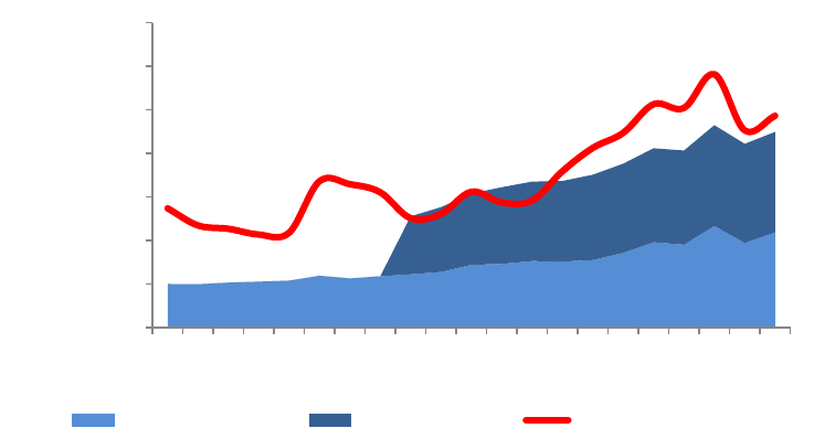
Figure 2 illustrates the drastic loss of sub-national fiscal autonomy, while Figure 3

illustrates the increase in their share of the expenditures. As can be inferred from both figures,

sub-national governments, and states in particular, have gained substantially greater expenditure

authority without acquiring further revenue-generating responsibilities. The heavy dependence

of the states on federal transfers has turned the federal government into their lender of last resort,

with the attendant moral hazard and risks for the federal budget.

2

SHCP. Estadísticas Oportunas de Finanzas Públicas y Deuda Pública. México, 2010.

3

IMCO. Índice de Competitividad Urbana 2010: Acciones urgentes para las ciudades del futuro. México, 2010.

5

Figure 2. State Revenues Raised by the Federal Government, 1989-2008

(as percent of total)

Source: IMCO with data from INEGI.

Figure 3. Distribution of General Government Expenditures, 1989-2007

(as percent of total)

Source: IMCO with data from INEGI.

Only four out of 32 state governments in Mexico finance more than 10 percent of their

expenditures (a low margin in itself) through own revenues. Table 1 ranks the 31 states plus the

Federal District by their degree of fiscal autonomy (defined as local taxes, rights, royalties, and

other local fees as a percentage of their total revenues).

60%

65%

70%

75%

80%

85%

90%

95%

1989

1990

1991

1992

1993

1994

1995

1996

1997

1998

1999

2000

2001

2002

2003

2004

2005

2006

2007

2008

0%

10%

20%

30%

40%

50%

60%

70%

80%

90%

100%

1989

1990

1991

1992

1993

1994

1995

1996

1997

1998

1999

2000

2001

2002

2003

2004

2005

2006

2007

2008

Municipalities State Governments Federal Government

6

Table 1. Sub-national Fiscal Autonomy, 2009

(own revenues as percent of total revenues)

33.0%

Distrito Federal

19.2%

Chihuahua

15.2%

Nuevo León

14.3%

Baja California Sur

9.4%

Guanajuato

8.5%

Baja California

7.7%

Campeche

7.4%

Sinaloa

6.9%

Hidalgo

6.9%

México

6.7%

Jalisco

6.3%

Tamaulipas

6.0%

Veracruz

5.8%

Chiapas

5.5%

Durango

5.5%

Aguascalientes

5.4%

San Luis Potosí

5.3%

Colima

4.9%

Yucatán

4.7%

Michoacán

4.3%

Puebla

3.9%

Morelos

3.5%

Guerrero

3.5%

Nayarit

3.4%

Tabasco

3.1%

Oaxaca

2.6%

Tlaxcala

Source: IMCO with data from the states’ budget laws.

If we consider that the federal government finances 92 percent of the state

governments’ budgets, and that 33 percent of federal revenues come from the oil industry

while sub-national governments have little say on oil policies, the following question

arises: how does oil dependence affect state governments? Using a straightforward

calculation with the mathematical formulas from the Fiscal Coordination Law, and holding

constant other variables,

4

a decrease in the price of a barrel of oil by US$2.00 should

represent an average decrease of 0.74 percent in State revenues through federal transfers.

However, given the requirement that federal transfers should be at least equivalent to the

amount calculated the prior year, this reduction is entirely absorbed by the Federal

government through spending cutoffs or increases in its debt, rather than passed on to the

subnational governments.

Although, municipalities have significantly greater fiscal autonomy than states, as

can be seen in Figure 4, the capacity of the third level of government to raise its own

resources has also declined over time, and has been replaced by federal transfers. In 1989,

4

Daily oil barrel production, estimated annual oil barrel price, oil barrel exportation, USD-MXN exchange

rate, revenue from the income tax, revenue from the value added tax, and revenue from the business tax.

7

municipalities raised 39 percent of their own revenues. By 2009, this had declined to an

average of 19 percent, as they came to depend increasingly on federal or state transfers,

which increased their vulnerability to unpredictable fluctuations in the oil market.

Figure 4. Federal and State Transfers to Municipalities, 1989-2009

as a Percent of Total Revenue

Source: IMCO with data from INEGI.

Mexico’s Fiscal Coordination Law and its political structure make it virtually

impossible to precisely identify the amount of oil revenues that are transferred to

municipalities. The Fiscal Coordination Law allows each state to determine the mechanism

for the distribution of federal transfers to its municipalities. Until 2010, for example, the

state of Chihuahua lacked a formula for calculating such transfers. Instead, the amount to

be transferred to each municipality was determined by a legislative decree. However, even

if municipalities could be subject to some degree of uncertainty regarding their share of oil

revenues, they are still protected by the restrictions stipulated in the Fiscal Coordination

Law.

The Fiscal Coordination Law establishes that federal transfers to sub-national

governments, regulated by a formula, cannot be reduced. Furthermore, the Fiscal

Coordination Law dictates that federal transfers to states be at least the same as the amount

calculated the prior year. The only reasons that federal transfers can decrease are: i) a fiscal

crisis wherein the national income is less than the year before, in which case the state

40%

45%

50%

55%

60%

65%

70%

75%

1989

1990

1991

1992

1993

1994

1995

1996

1997

1998

1999

2000

2001

2002

2003

2004

2005

2006

2007

2008

2009

8

governments would receive the same proportion of the total federal budget as the prior

year, but a smaller quantity of funds; or ii) a decrease in the country or the state’s

population. Hence, as can be seen in Figure 5, federal transfers to sub-national governments

are influenced little by decreases in oil revenue. As a matter of fact, from 1990 to 2010,

federal transfers to sub-national governments grew by 194 percent. Total national revenue

from oil grew at a much slower pace, 83 percent, in the same period.

As the situation stands today, the federal government passes almost all of its oil

revenue to the sub-national governments. Indeed, from 1998 to 2003, revenue from oil

alone would have been insufficient to cover federal transfers to sub-national governments

(Figure 5). Additionally, under current circumstances, every reduction in oil prices is

absorbed by the federal government. That means that, in the case of a US$2.00 reduction in

oil prices, in order to fulfill restrictions of Fiscal Coordination Law, Federal government

would have to offset a reduction of 0.49 percent in municipal revenues. Combined with the

amount corresponding to states, this represents a reduction in the federal budget of 1

percent.

Figure 5. Oil Revenue vs. Federal Transfers

(in constant MXN millions)

Source: IMCO with data from INEGI and the Treasury Ministry (SHCP).

$-

$200,000

$400,000

$600,000

$800,000

$1,000,000

$1,200,000

$1,400,000

1990

1991

1992

1993

1994

1995

1996

1997

1998

1999

2000

2001

2002

2003

2004

2005

2006

2007

2008

2009

2010

PARTICIPACIONES APORTACIONES REVENUE FROM OIL

9

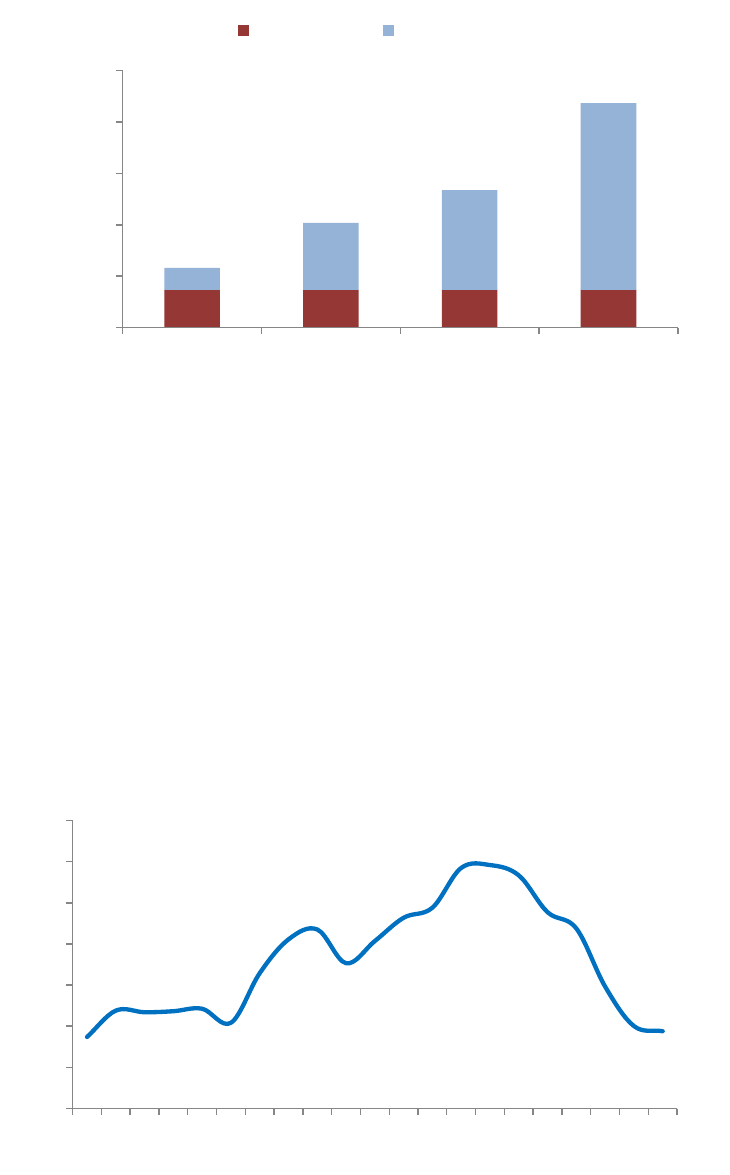
At first glance, such declines might not seem very drastic. However, history has

shown that oil prices tend to fall by much more than US$2.00 (Table 2). For example, in

1998 the average price of oil per barrel was 34 percent less than the price assumed in the

budget law. According to estimations by IMCO, using data from the economic criteria

forecasts published by the central government and the Law on Hydrocarbons, a decline of

US$10.00 in the budgeted price per barrel of oil would reduce the national budget by 5

percent. Figure 6 shows that the loss of revenue from such a decline would be equivalent to

two-thirds of the total public debt. To offset this loss, the base for the value-added tax

would have to be increased by 36 percent, or the rate would have to increase from 16

percent to 22 percent.

Table 2. Projected vs. Actual Oil Prices per Barrel,

1998-2008 Annual Averages

Official Expected

Oil Barrel Price

(USD)

Year Average

Oil Barrel Price

(USD)

Difference ( percent)

1998

$15.50

$10.18

-34

1999

$9.25

$15.57

68

2000

$15.00

$24.79

65

2001

$18.00

$18.61

3

2002

$15.50

$21.52

39

2003

$18.35

$24.77

35

2004

$20.00

$31.05

55

2005

$23.00

$42.71

86

2006

$36.50

$53.05

45

2007

$42.80

$61.63

44

2008

$49.00

$89.38

82

Source: IMCO with data from Pardinas (2009).

10

Figure 6. Impact of a US$10.00 per Barrel Decrease in Price of Oil

on the Federal Budget, 2010 (in MXN millions)

Source: IMCO with data from federal budget laws for 2010.

Note: Percentages represent the reduction of revenue due to a $10 USD loss.

Once the relationship between oil revenue and the Mexican governments’ finances

has been established and understood, a second question emerges. How feasible is a crisis

scenario in the Mexican oil industry? The answer is that it is a latent possibility. Figure 7

illustrates the perilous recent history of Mexico’s oil production. As of 2009, average daily

production of oil has fallen by 23 percent from its peak in 2004 and is now at production

levels similar to those observed in the early 1980s.

Figure 7. Daily Crude Oil Production, 1990-2010

(in thousands of barrels)

Source: IMCO with data from PEMEX.

$0

$200,000

$400,000

$600,000

$800,000

$1,000,000

Public Debt Value Added Tax Income Tax Oil

$10 USD Loss Revenue

2200

2400

2600

2800

3000

3200

3400

3600

1990

1991

1992

1993

1994

1995

1996

1997

1998

1999

2000

2001

2002

2003

2004

2005

2006

2007

2008

2009

2010

63%

36%

27%

17%

11

Estimates from the Mexican Institute of Competitiveness, based on a conservative

calculation of the behavior of oil demand and the decrease in production from oil deposits,

indicate that Mexico will become a net importer of crude oil by the year 2017 (Figure 8).

From then on, oil revenue will likely be replaced by oil expenditures. Under that scenario,

the Fiscal Coordination Law’s prohibition on reducing transfers in nominal terms might not

be sustainable; sub-national governments would be forced to find ways of raising revenues

independently to replace dwindling federal transfers.

Figure 8. Crude Oil Production and Demand, 2005-2025

(in thousands of barrels)

Source: IMCO estimates with data from PEMEX. *Estimated

3. Fiscal Autonomy of the States

Federal transfers to states are funded by federal taxes and royalties from oil revenues. They

are of two types: revenue sharing (Participaciones) and special purpose grants

(Aportaciones) which are earmarked for specific social services such as education, health

and public safety. These transfers have a horizontal nature, which means that subnational

units receive a pre-determined percentage of such transfers regardless of their individual

contributions to the fund (Recaudación Federal Participable). The initial objective of this

structure was to transfer resources from wealthier states to poorer states in order to promote

1500

1750

2000

2250

2500

2750

3000

3250

3500

2005

2006

2007

2008

2009

2010

2011*

2012*

2013*

2014*

2015*

2016*

2017*

2018*

2019*

2020*

2021*

2022*

2023*

2024*

2025*

12

development. However, this structure has been counterproductive in regard to local tax

collection.

Aside from taxes that only the central government can collect, there are a variety of

taxes that can be introduced by state governments. However, each state decides the number,

coverage of the base, and rate structure for each tax, thus determining the amount of

potential revenue that could be raised.

Table 3. Number and Taxes of Each State for 2010

State

Number

of taxes

Payroll

tax

Lodging

tax

Tax on

lotteries

Tax on

acquisition

of used

motor

vehicles

Tax on

vehicle

ownership

Leisure and

entertainment

tax

Others

Aguascalientes

7

*

Baja California

8

*

Baja California Sur

4

*

Campeche

7

*

Coahuila

7

*

Colima

7

*

Chiapas

7

*

Chihuahua

9

*

D.F.

7

*

Durango

6

*

Guanajuato

7

*

Guerrero

9

*

Hidalgo

7

*

Jalisco

8

*

México

4

*

Michoacán

4

*

Morelos

9

*

Nayarit

12

*

Nuevo León

4

*

Oaxaca

8

*

Puebla

6

*

Querétaro

8

*

Quintana Roo

6

*

13

Table 3., continued

State

Number

of taxes

Payroll

tax

Lodging

tax

Tax on

lotteries

Tax on

acquisition

of used

motor

vehicles

Tax on

vehicle

ownership

Leisure and

entertainment

tax

Others

San Luis Potosí

7

*

Sinaloa

4

*

Sonora

5

*

Tabasco

6

*

Tamaulipas

5

*

Tlaxcala

8

*

Veracruz

5

*

Yucatán

7

*

Zacatecas

5

*

Source: IMCO with data from State Revenue Acts.

Between 2000 and 2008, tax revenue represented 42 percent of own state revenues,

while non-tax revenue (rights, land use, products, royalties, etc.) contributed the remaining

58 percent. The most important state tax is the payroll tax. In 2008, it represented 63.3

percent of the states’ total tax revenue. Its importance lies in the breadth and stability of its

tax base. This tax was introduced gradually across states, and since 2008, all states have

collected it. However, the tax regime is not the same in all the states; the main source of

variance is the difference in rates, which range between 1 and 2 percent.

Figure 9. Composition of States’ Total Tax Revenue, 2008

Source: IMCO with data from INEGI.

63.3%

28.1%

4.2%

4.4%

Payroll tax Direct taxes (excluding payroll tax) Indirect taxes Other taxes

14

As in the case of tax revenues, non-tax revenues take a variety of forms, and their

application varies across states. Among non-tax revenues, fees or derechos (mainly for

public and private transportation, business or property registration, civil registration, and

city services) are the most significant source of revenue, contributing 34 percent of local

revenues. The rest of local revenues are generated by capital gains, tax penalties, and

surcharges.

The tax on vehicle ownership deserves special mention because of recent legislative

changes. This tax is collected by the central government according to the vehicle registry of

each state. However, the revenue raised by this tax is returned to the state where the

vehicle is legally registered. In 2008, revenues from this tax represented 1.8 percent of total

states’ revenues, but this share varies among the states (Figure 10). This tax has been in

place since 1961, but in 2012, a federal decree removing it will take effect. However, the

decree allows the states to adopt it as a local tax.

Figure 10. Tax on Vehicle Ownership

as a Percent of Total Revenue, 2008

Source: IMCO with data from the Ministry of the Treasury and INEGI.

0.0%

0.5%

1.0%

1.5%

2.0%

2.5%

3.0%

3.5%

4.0%

4.5%

5.0%

Nuevo León

D. F.

Jalisco

Querétaro

Quintana Roo

Aguascalientes

Guanajuato

Baja California

Sinaloa

Yucatán

Coahuila

Sonora

México

Puebla

Tamaulipas

Chihuahua

San Luis Potosí

Colima

Morelos

Baja California Sur

Michoacán

Veracruz

Campeche

Durango

Tabasco

Hidalgo

Nayarit

Zacatecas

Guerrero

Chiapas

Tlaxcala

Oaxaca

15

4. Determinants of the Fiscal Effort of Mexican States: A Stochastic

Frontier Analysis

Most of the literature on fiscal effort consists of empirical studies. In this section we will

propose a stochastic frontier model for taxation capacity that will allow us to measure the

revenue-collecting effort of Mexican states, defined as the ratio of observed tax collection

to the potential collection at the efficiency frontier. Such frontiers establish a potential tax

collection given the fiscal unit economic characteristics and legal framework.

This exercise involving two procedures has been recognized as a useful but

inconsistent one mainly because of the underlying independence assumption. Battese and

Coeli (1985) proposed the model that will be used in this working paper to address that

issue.

In order to estimate the maximum likelihood estimators of the parameters, the

stochastic frontier estimation method consists of three steps:

1. First, we obtain the function Ordinary Least Squares estimators (OLS)

that produces parameters 



  All parameters will be unbiased with

the exception of the intercept 



.

2. Using the 



,    parameters and the 



and 



parameters adjusted

according to the corrected ordinary least squares formula proposed by

Coelli (1995), a two-stage grid search of the  parameter is conducted.

If there is any other parameter, it is set to zero in this stage.

3. To obtain the maximum likelihood estimators we use the values selected

in the grid search as starting values in an iterative maximization

procedure. Since we will use the software Frontier 4.1, this procedure

will be the Davidon-Fletcher-Powell Quasi-Newton method.

In order to explain the differences among states regarding government effort in tax

collection, the model includes some economic variables such as GDP per capita, the share

of industrial output in GDP, a coefficient of income inequality, and a measure of the

informal economy, which does not pay payroll taxes or fees for services (water, electricity,

etc.). We include fiscal variables, such as the share of central government transfers in total

revenue and public investment expenditure. We also consider political variables, such as

16

the governor’s political affiliation, and institutional variables, such as corruption and a good

governance index.

Given these assumptions, the model specification for the tax collection potential

(the stochastic frontier for total state tax revenues per capita) is the following:





  



 







  







  



, (1)

Similarly, we define the payroll tax function as follows:





  



 







  







  



, (2)

where:





 Tax collection per capita in state  in year 





 Payroll tax collection per worker in state  in year 





 Economically active population (in both the formal and informal sector) as share

of total population of state  in year 





 GDP per capita in state  in year 





 Error term defined as follows:





 



 



, (3)

where the 



are random variables, which are assumed to be independent and identically

distributed (iid)  





 and independent of the 



that are non-negative random

variables, assumed to account for technical inefficiency

5

in revenue raising and to be iid as

truncations at zero of the 



 





 distribution where 



 



 and 



is a   

vector of variables which may influence the effort of a local government and  is a   

vector of parameter to be estimated. The panel of data need not be complete.

With the calculation of the maximum likelihood estimator in mind, we will replace







and 





with 











 



and we define  



















as did by Battese and Corra

5

Through this document the term “efficiency” will be substituted for “effort” since it makes more sense when

talking about government tax collection.

17

(1977). Note that    and thus this range can be searched to provide a good starting

value for use in an iterative maximization process.

Given the assumptions stated above regarding the error term, for (1) we define:





 



 







  







  







  







  



,

Similarly, for (2) we define:





 



 







  







  







  







  







  



,

where:





 Share of industrial GDP in the GDP of state  in year 





 Institutional Quality of Justice Index in state  in year

6





 Dummy that is 1 if the governor of state  in year  belongs to the political party of

the president and is 0 otherwise





 Informality rate in state  in year 





 Corruption and Good Government Index of state  in year 





 Transparency Index of state  in year 





 Error term

For both models, observations are for eight years (from 2001 to 2008). For (1) we

use a balanced panel with 256 observations, while for (2) we use an unbalanced panel with

216 observations, since during this period some states did not have a payroll tax and they

implemented it gradually.

Ex ante, for both functions we expect a positive sign in the two independent

variables, since the greater the economically active population or the economy’s output per

capita, the higher revenues should be. We also expect a positive sign for institutional

quality of justice and for the transparency index, since the greater the government

6

Consejo Coordinador Financiero, “Ejecución de Contratos Mercantiles e Hipotecas en las Entidades

Federativas Mexicanas.”

18

accountability perceived by the citizens, the more willing they are likely to be to pay taxes.

For the share of industrial GDP a positive sign is also expected, since it is easier to collect

from this sector. If the governor has the same political affiliation as the president, a

negative relation is expected, since we assume they would be favored with discretionary

transfers. Moreover, negative signs are expected for the informality rate and the corruption

and good governance index.

In order to determine if a stochastic frontier function is required, we tested the

significance of the  parameter. For both models, the result determined that the null

hypothesis (that  equals zero) would be rejected, indicating that 





is not zero, and hence

the 



should not be removed.

5. Analysis of Empirical Estimates

The robust variable of the model (1) is the GDP per capita, while for the effort measure of

this model, the industrial contribution to the total output and the corruption index were

significant and with the expected sign.

Table 4. Maximum Likelihood Estimators for the State Revenue Model

Coefficient

Standard-

error

t-ratio

P-value

beta 0

-13,99

0,87

-16,17

0,000

***

beta 1

0,68

1,39

0,49

0,627

***

beta 2

1,72

0,11

16,31

0,000

***

delta 0

-1,32

0,66

-1,99

0,047

***

delta 1

0,25

0,22

1,10

0,271

***

delta 2

7,61

1,08

7,03

0,000

***

delta 3

-0,00

0,01

-0,76

0,445

***

delta 4

-0,12

0,04

-2,87

0,004

***

sigma-squared

0,87

0,17

5,13

0,000

***

gamma

0,94

0,03

32,57

0,000

***

Significant 99%.

**

Significant 95%.

*

Significant 90%.

Source: Authors’ calculations.

19

Table 5. Mexican States’ Tax Collection Effort, 2001-2008 (percent)

State

2001

2002

2003

2004

2005

2006

2007

2008

Aguascalientes

9.5

10..8

11.8

13.5

18.4

34.3

56.4

55.5

Baja California

53.7

61.6

65.6

68.1

69.0

70.0

74.7

76.5

Baja California

Sur

50.5

37.1

47.8

50.9

76.1

83.3

86.0

85.8

Campeche

0.8

0.9

1.1

1.3

1.5

2.1

2.3

Chiapas

27.5

30.5

66.4

79.9

81.3

84.9

89.1

91.0

Chihuahua

77.0

78.8

79.0

77.9

79.5

80.6

82.3

82.6

Coahuila

20.7

22.4

19.9

20.2

22.4

21.7

24.3

26.7

Colima

10.8

11.8

12.0

12.1

49.3

55.4

61.4

60.4

Distrito Federal

88.5

89.1

88.5

90.4

89.5

89.1

89.9

Durango

33.0

36.4

38.5

35.0

38.7

64.9

67.9

67.8

Guanajuato

10.2

8.7

7.4

9.0

59.5

68.4

73.1

78.1

Guerrero

79.4

80.6

83.9

72.6

87.1

89.5

89.1

91.1

Hidalgo

28.6

29.4

47.1

50.4

55.5

66.2

65.0

80.6

Jalisco

44.9

47.6

49.2

50.3

53.4

54.7

57.4

60.7

México

72.9

82.5

81.9

79.8

83.4

91.2

91.6

Michoacán

16.9

19.2

45.6

56.1

65.4

68.7

64.4

Morelos

17.3

20.3

21.3

21.9

28.9

29.9

53.3

72.7

Nayarit

55.5

76.7

79.4

85.1

85.8

81.7

89.3

89.5

Nuevo León

33.7

35.7

36.1

35.3

37.1

36.5

35.6

39.2

Oaxaca

10.9

27.7

38.8

36.9

47.7

61.6

61.8

66.8

Puebla

36.6

46.9

51.2

48.2

48.0

65.1

73.3

75.0

Querétaro

12.6

15.1

14.6

14.1

61.8

74.1

74.0

77.5

Quintana Roo

52.2

53.9

62.4

67.0

65.5

66.9

72.1

79.4

San Luis Potosí

19.1

19.0

22.2

35.2

35.8

36.9

46.8

61.3

Sinaloa

33.2

35.2

38.1

37.8

41.0

46.4

47.2

60.3

Sonora

53.1

59.1

49.8

48.8

54.6

50.6

57.4

59.5

Tabasco

6.2

6.9

7.8

7.9

8.4

8.5

8.3

7.5

Tamaulipas

43.5

45.0

45.9

41.4

43.7

50.8

49.2

52.9

Tlaxcala

49.8

58.8

66.2

65.9

74.4

75.6

74.4

79.2

Veracruz

43.8

71.3

66.2

67.7

69.5

67.1

66.0

68.5

Yucatán

44.0

46.6

52.2

48.6

51.9

62.8

59.0

63.7

Zacatecas

58.3

66.0

67.5

65.8

73.4

75.7

79.8

80.9

Source: Authors’ calculation.

On average, tax collection effort increased by 29.5 percentage points between 2001

and 2008, from 37.3 percent to 66.8 percent, while average tax collection per capita

increased by 68.9 percent from MXN 221 in 2001 to MXN 374 in 2008. Using this

20

information and that provided by the model showing a positive relation between GDP and

tax collection, we can assume that growth in tax revenue is largely due to Mexico’s

economic growth before the 2008 crisis and to increased government tax effort during this

period.

7

For illustrative purposes, we will divide the states into three groups. In the first one

we will include those states whose average effort within this period is between the mean

and one standard deviation (  ), in the second one we will include those states whose

average effort is below one standard deviation (  ), and in the third one we will include

those states with average effort above one standard deviation (  ).

Figure 11. Spatial Distribution of Effort, 2001-2008 Average

Source: Authors’ compilation.

7

Between 2001 and 2008, the Mexican economy recorded cumulative real growth of 21 percent.

21

For a deeper analysis, we will divide Mexican states into four groups (Figure 12).

8

This division will allow us to distinguish between those states that have low tax collection

per capita because of their lack of effort from those which have low tax revenue because of

their narrow and limited tax base. Moreover, this distinction will also allow us to

distinguish between those states whose tax collection per capita is high because they make

an efficient tax effort from those which have high tax collection per capita because of

favorable economic conditions rather than collection efforts.

Figure 12. Mexican States’ Collection Effort vs. Tax Collection per Capita, 2008

Source: Authors’ calculations.

There is no surprise in regard to the states in Quadrants I and III, since we assume a

direct relation between effort and tax revenues. States in Quadrant II are those whose tax

collection effort is large, but they are not collecting much revenue from taxes. Quadrant II

includes Durango, Guerrero, Jalisco, Puebla, Tlaxcala, Veracruz, Yucatán, and Zacatecas.

The causes may be different for each state and may include issues such as ill-defined tax

8

For this analysis we exclude Distrito Federal since it is an outlier because of its different and broader taxing

powers and responsibilities.

77%

86%

2%

91%

83%

27%

68%

78%

91%

81%

92%

64%

73%

89%

39%

67%

75%

78%

79%

61%

60%

59%

7%

53%

79%

69%

64%

81%

0%

10%

20%

30%

40%

50%

60%

70%

80%

90%

100%

0 100 200 300 400 500 600 700 800

Tax Collection Effort

Tax Collection per Capita, MX pesos

Quadrant I

Quadrant II

Quadrant III

Quadrant IV

22

bases, many special regimes, or many exemptions, which restrict their possibility frontier.

The recommendation for these states is to promote structural changes in their taxation

systems.

On the other hand, Campeche,

9

Nuevo Leon, Sonora, and Tamaulipas are in

quadrant four: despite their low tax effort, they have a high tax collection per capita. These

states have a high potential for improvement since they seem to be exploiting their tax base

correctly. For Campeche, this phenomenon is caused by the large contribution of oil

production to its total output. For the other cases, this might be due to the large number of

firms that have decided to locate their logistics centers there because of its convenient

geographic location, thus facilitating tax collection with little effort. A hypothetical flight

of capital from the state could leave these states in dire financial straits since more than 10

percent of total revenue is own revenue. But at the same time, additional tax collection

effort by the government could generate significant additional revenue.

Figure 12. Mexican States’ Effort and Tax Collection per Capita, 2008

Source: Authors’ compilation.

Note: TCE refers to tax collection effort while TRPC refers to tax revenue per capita.

9

From here on, the analysis will not consider this state unless otherwise specified, since almost 85 percent of

its total output is due to oil.

23

With respect to the results of the model defined in (2) for the payroll tax function,

the results point in the same direction as those obtained for the total revenue function.

Once again, the robust variables include GDP per capita and for this model’s error term

almost all the variables were significant (except the corruption index) and with the expected

sign.

Table 6. Maximum Likelihood Estimators for the Payroll Tax Model

Coefficient

Standard-

error

t-ratio

P-value

beta 0

-13.13

0.96

-13.72

0.000

***

beta 1

-2.00

1.28

-1.56

0.119

***

beta 2

1.76

0.10

16.82

0.000

***

delta 0

-5.21

0.98

-5.32

0.000

***

delta 1

-8.08

1.98

-4.09

0.000

***

delta 2

8.17

0.85

9.60

0.000

***

delta 3

-0.05

0.03

-1.54

0.124

***

delta 4

1.46

0.32

4.62

0.000

***

delta 5

-1.39

0.38

-3.62

0.000

***

sigma-squared

0.48

0.07

6.91

0.000

***

gamma

0.66

0.06

11.10

0.000

***

Significant 99%.

**

Significant 95%.

*

Significant 90%

Source: Authors’ calculations.

As before, we compute the effort of Mexican states in payroll tax collection. The

results are shown in Table 7.

Table 7. Mexican States’ Effort for Payroll Tax Collection, 2001-2008 (percent)

State

2001

2002

2003

2004

2005

2006

2007

2008

Aguascalientes

N/A

63

87

90

Baja California

N/D

89

88

87

88

89

Baja California

Sur

76

78

82

85

89

91

89

Campeche

2

3

4

Chiapas

89

90

94

93

92

Chihuahua

85

84

86

84

82

86

87

Coahuila

N/D

46

43

48

36

39

44

Colima

N/A

79

77

82

85

Distrito Federal

92

93

91

90

92

Durango

59

63

65

62

67

68

72

74

24

Table 7., continued

State

2001

2002

2003

2004

2005

2006

2007

2008

Guanajuato

N/A

90

87

88

89

Guerrero

92

N/D

90

88

92

91

92

Hidalgo

76

72

80

77

81

73

74

84

Jalisco

92

93

92

90

91

92

México

N/D

91

90

91

89

92

Michoacán

N/D

87

89

91

90

Morelos

N/A

89

92

Nayarit

87

91

93

69

81

85

Nuevo León

87

88

87

75

74

59

64

75

Oaxaca

N/D

82

87

86

89

84

85

89

Puebla

N/D

89

88

91

92

Querétaro

N/A

87

90

88

89

Quintana Roo

87

88

87

83

89

90

San Luis Potosí

69

67

68

87

88

82

85

88

Sinaloa

83

84

85

84

80

84

Sonora

N/D

65

N/D

Tabasco

19

16

18

17

15

12

11

9

Tamaulipas

80

79

80

77

75

79

83

Tlaxcala

90

91

93

92

95

94

Veracruz

91

93

91

90

89

Yucatán

86

91

90

91

93

92

90

Zacatecas

81

82

78

80

81

80

Source: Authors’ calculation. N/A corresponds to cases in which the payroll tax

was not yet implemented in the state. N/D corresponds to cases in which there

was no official information available.

Table 7 shows that considerable effort is made to collect this tax in most states, and

has grown from 76.2 percent in 2001 to 81.1 percent in 2008, on average.

Using the data provided in Tables 5 and 7, we can divide the states into four groups.

25

Figure 13. Total Tax Collection Effort vs. Payroll Tax Collection Effort, 2008

10

Source: Authors’ calculation.

In Quadrant II are states such as Colima, Guanajuato, and Querétaro. They

implemented payroll taxes in 2005 as a source of sub-national revenue. The results suggest

that implementation of the payroll tax was successful, since their payroll tax collection

effort is high. However, the results also suggest that they overestimate its potential. These

three states are among the 10 with the lowest share of payroll tax in total revenue. These

states have room for improvement and can focus on the collection of other taxes so they can

increase their revenue. Also in this quadrant is Mexico City, which, although it has

different taxation powers and is exploiting the payroll tax efficiently, still has significant

opportunities for improvement in the collection of other taxes.

In quadrant four are states such as Durango and Zacatecas, which are also among

those states where the contribution of the payroll tax to total revenue is lowest. The results

suggest that even though these states are efficient in general with respect to total tax

collection, they have not managed payroll taxes properly, focusing their efforts instead on

10

Data for Sonora correspond to 2006, the latest available data.

40.0%

50.0%

60.0%

70.0%

80.0%

90.0%

100.0%

20.0% 30.0% 40.0% 50.0% 60.0% 70.0% 80.0% 90.0% 100.0%

Payroll tax effort

Total tax collection effort

Quadrant I

Quadrant II

Quadrant III

Quadrant IV

26

the collection of all other taxes. States in quadrants one and three have the expected

behavior: we expected a positive correlation between the effort in total tax collection and

effort regarding payroll tax collection.

For both models, it was surprising that employment was not a significant variable.

In the results of (1), EAP has a positive but not significant sign. This may suggest that

policies should be focusing on creating better-remunerated jobs rather than more low value-

added positions. The result of (2) is even more interesting, since it shows a negative

relationship between payroll tax and employment that is very close to the significance zone.

Some authors state that the payroll tax is a burden on a productive factor (labor) that

discourages the use of this factor in the formal sector. Even though this is a relevant and

quite important issue, it is beyond the scope of this project and requires further research.

6. Revenue Potential for Mexican States

What would happen if all states operated with 100 percent effort? In the following section

we will use the data obtained before to discuss a hypothetical scenario facing Mexican

states if they could raise all of the potential revenue.

First, we define the Fiscal Autonomy Index (FAI) as follows:

 









, (4)

where





 Total revenue of state  in year 





 Own revenue of state  in year including not only tax revenue but other local

revenue as well.

The FAI tells us what proportion of total revenue is contributed by sub-national

governments. For this analysis, we will use 2008 data. Since no state has tax collection

that is 100 percent efficient, the potential FAI will be greater than the actual one. The

potential autonomy index will be computed by using potential tax collection in both total

revenue and own revenue.

27

Figure 14. Fiscal Autonomy Index, 2008

Source: Authors’ calculations.

Even if the potential is raised, fiscal autonomy will not increase significantly. The

FAI average would rise from 8.0 percent to 11.1 percent, suggesting that the weight of

central government transfers would remain very high. This is even more worrisome if we

exclude Mexico City and Campeche, since without them the average would only rise from

7.1 to 8.6 percent.

If we sort Mexican states according to their degree of fiscal autonomy and compare

the actual situation with the potential one, the state that would benefit the most in relative

terms is Tabasco, climbing almost 20 places,

11

followed by Coahuila and Tamaulipas,

advancing eight and three places, respectively. In the other direction, changes would not be

so dramatic, since those states that would fall in ranking would only do so by one or two

places.

At first, this would not create much additional revenue for the states, but given that

an important percentage of Participaciones distributed to the states depends on its own tax

collection efforts, those states for whom revenue increases more significantly would be

11

Tabasco is also one of the most important oil producers in the country, which is why, as in the case of

Campeche, the results are overstated.

0

0.05

0.1

0.15

0.2

0.25

0.3

0.35

0.4

Distrito Federal

Nuevo León

Chihuahua

Queretaro

Baja California

Quintana Roo

Tamaulipas

Coahuila

Tabasco

Sonora

Mexico

Baja California…

Sinaloa

Jalisco

Guanajuato

Aguascalientes

Hidalgo

Zacatecas

San Luis Potosí

Durango

Chiapas

Morelos

Michoacan

Puebla

Colima

Yucatan

Veracruz

Nayarit

Tlaxcala

Oaxaca

Guerrero

Potential FAI

Real FAI

28

rewarded in the next central government transfer allocation through the revenue-sharing

mechanism.

Even if all states raised their potential revenue and considering the situation faced

by Tabasco, the last three states would stay the same. This suggests that their dependence

on central government transfers would remain the same, as if they had made no extra effort

at all.

On average, states’ own revenue would only increase by 11.5 percent, and the share

of states’ own revenue in total tax revenue would increase from 41.2 to 56.1 percent.

Improving states’ efforts with their current tax bases would not be sufficient to substantially

strengthen the states’ public finances.

Figure 15. Share of Potential Tax Revenue in Potential States’ Own Revenue

Source: Authors’ calculations.

0 0.2 0.4 0.6 0.8

Campeche

Distrito Federal

Nuevo León

Chihuahua

Queretaro

Baja California

Quintana Roo

Tamaulipas

Coahuila

Tabasco

Sonora

Mexico

Baja California Sur

Sinaloa

Jalisco

Guanajuato

Aguascalientes

Hidalgo

Zacatecas

San Luis Potosí

Durango

Chiapas

Morelos

Michoacan

Puebla

Colima

Yucatan

Veracruz

Nayarit

Tlaxcala

Oaxaca

Guerrero

Current share

Potential Share

29

Table 8. Increase in States’ Own Revenue Assuming 100 Percent Effort, 2008

State

Increase (%)

Aguascalientes

33.32

Baja California

13.60

Baja California

Sur

7.84

Campeche

1795.14

Chiapas

2.58

Chihuahua

6.83

Coahuila

79.64

Colima

28.57

Distrito Federal

5.51

Durango

19.75

Guanajuato

13.15

Guerrero

5.39

Hidalgo

8.77

Jalisco

28.03

México

3.25

Michoacán

17.34

Morelos

14.37

Nayarit

7.14

Nuevo León

54.89

Oaxaca

9.90

Puebla

14.53

Querétaro

12.99

Quintana Roo

10.51

San Luis Potosí

25.63

Sinaloa

15.42

Sonora

19.98

Tabasco

256.01

Tamaulipas

37.75

Tlaxcala

8.18

Veracruz

23.62

Yucatán

29.15

Zacatecas

4.88

Source: Authors’ calculation.

Moreover, under the assumption of 100 percent effort by all states, the increase in

the states’ total revenue would be negligible.

30

Table 9. Increase in Total State Revenue Assuming 100 Percent Effort, 2008

State

Increase (%)

Aguascalientes

2.0

Baja California

1.5

Baja California

Sur

0.7

Campeche

134.7

Chiapas

0.2

Chihuahua

1.0

Coahuila

5.1

Colima

1.3

Distrito Federal

2.0

Durango

1.1

Guanajuato

1.0

Guerrero

0.2

Hidalgo

0.6

Jalisco

2.1

México

0.3

Michoacán

0.9

Morelos

0.8

Nayarit

0.3

Nuevo León

8.6

Oaxaca

0.4

Puebla

0.7

Querétaro

1.6

Quintana Roo

1.1

San Luis Potosí

1.4

Sinaloa

1.3

Sonora

1.8

Tabasco

8.4

Tamaulipas

3.2

Tlaxcala

0.3

Veracruz

0.9

Yucatán

1.1

Zacatecas

0.3

Source: Authors’ calculations.

We can see that most of the states would increase their total revenue by less than 2

percent. In fact, the average increase would be 5.8 percent but, if Mexico City and

Campeche are excluded, this average would be reduced to 1.7 percent. Moreover, even if

31

we assume a 100 percent effort and include Campeche’s figures, total own revenues would

grow by 33.7 percent, but total revenues would only grow by 3.5 percent.

The results suggest that state tax bases are in general being relatively well exploited,

especially the payroll tax base. The empirical evidence shows that the performance of

government institutions regarding revenue collection is generally acceptable. By comparing

the real and potential revenue of Mexican states, we can observe that there is not much

room for improvement in terms of tax collection. Given the current tax bases, even if they

could achieve their potential, the benefits would be very limited and would not provide

much in terms of total state revenues.

7. The Fiscal Autonomy of Municipalities

12

Fiscal centralism in Mexico has experienced historical ups and downs. In the late

nineteenth and early twentieth centuries, sub-national governments, both states and

municipalities, were relatively more important vis-à-vis the central government. In 1900,

municipal revenue exceeded 1 percent of GDP, but in the 1930s and 1940s, after the first

National Tax Convention, it decreased to about 0.5 percent of GDP.

13

The ratio of

municipal revenue has remained at this level for almost 70 years, and today it is actually

close to 0.4 percent of GDP (Figure 16). Mexico is at the bottom relative to OECD

countries, where the average revenue collection at this level of government is nearly 3

percent of GDP.

14

12

For this section, Mexico City is excluded from the analysis unless otherwise specified.

13

Díaz-Cayeros (2006: 37).

14

OCDE, Revenue Statistics 1965-2007.

32

Figure 16. Central Government, State and Municipal Tax Revenues

(as percent of GDP, 1990-2007)

Source: INEGI, World Bank, Díaz Cayeros (2006).

The main sources of municipal revenue are:

 Exploitation of capital assets

 Contributions enacted through local laws

 Fees for the provision of public services

 Central government transfers

Municipalities have no authority to decide which taxes to levy, although some

authority in this area is granted by local laws approved by state congresses. Municipalities

cannot create taxes and collect them on their own, but they can administer the revenue

sources that have been decided by local congresses. State revenue acts and state tax codes

regulate municipal tax bases.

Two of the pillars of municipal revenues are property taxes and water rights.

Between 2001 and 2008, property taxes accounted for almost 57 percent of municipal tax

revenues and more than 27 percent of own municipal revenues.

0%

2%

4%

6%

8%

10%

12%

1990

1991

1992

1993

1994

1995

1996

1997

1998

1999

2000

2001

2002

2003

2004

2005

2006

2007

Municipios

Estados y DF

Federación

Tax Coordination Law

Municipalities

State governments

Federal government

33

Figure 17. Composition of Own Municipal Revenues

(average, 2001-2008)

Source: IMCO with data from INEGI.

The expenditure decentralization policy has influenced property tax collection.

Rising central government transfers sapped incentives to collect taxes. In 2008, the central

government tried to reverse the situation by including economic efficiency criteria in the

revenue-sharing formula. Internationally, in 2008, Mexico was the OECD country with the

lowest property tax collection rate as a percentage of GDP.

27%

21%

25%

7%

18%

2%

Property tax Other taxex Rights Products Exploitations Contributions

34

Figure 18. Property Tax as Percent of GDP, 2008

Source: OECD revenue statistics.

Cadastral updates have significantly improved property tax collection. With the

changes in the agricultural legislation in 1992 and the updating of property values, the share

of property tax in total revenue reached 10 percent in 1994. However, it fell back to

previous levels subsequently, following the increase in federal transfers.

Figure 19. Share of Property Tax in Total Revenue

Source: IMCO with data from INEGI.

0

0.5

1

1.5

2

2.5

3

3.5

4

4.5

United Kingdom

Canada

France

Israel

Korea

United States

Japan

Luxembourg

Spain

Australia

Belgium

Iceland

Switzerland

Denmark

Italy

New Zealand

Ireland

OECD - Total

Netherlands

Greece

Portugal

Chile

Norway

Poland

Finland

Sweden

Germany

Hungary

Turkey

Slovenia

Austria

Czech Republic

Slovak Republic

Mexico

5.5%

6.0%

6.5%

7.0%

7.5%

8.0%

8.5%

9.0%

9.5%

10.0%

10.5%

1989

1990

1991

1992

1993

1994

1995

1996

1997

1998

1999

2000

2001

2002

2003

2004

2005

2006

2007

2008

2009*

Tax Coordination Law

35

In 2008, 537 of the 2,456 municipalities (22 percent) did not levy property taxes or

did not report doing so. Eighty percent of all property tax revenue was collected by only

105 municipalities (4 percent). In fact, only 29 of the more than 2,400 municipalities

collect more than 50 percent of their total revenue; the rest depend on transfers from their

states or the central government.

Figure 20. Distribution of Own Municipal Revenues

as a Percent of Total Expenditure, 2008

Source: IMCO using data from INEGI.

Municipalities have a potential margin in revenue capacity that has not been fully

exploited. These are property taxes and water rights. However, land records and the tap-

water infrastructure would need to be updated. Even if not intended to become a source of

income, water rights should cover at least the cost of provision, to avoid giving rise to

deficits.

Given municipalities’ limited access to credit, the share of debt in total revenues

chas remained below 10 percent and has followed a downward trajectory. There is a

possibility to raise resources through debt, but the rules and circumstances under which

debt can be incurred would need to be established, since even in local laws, different

criteria are applied with respect to municipal debt contracting.

1561

439

208

135

66

20

9

0% - 9% 10% - 19% 20% - 29% 30% - 39% 40% - 49% 50% - 59% more than

60%

36

Added to this, municipalities have another issue to solve. Mayors in Mexico serve

only three-year terms, one of the shortest in Latin America, and immediate re-election is

prohibited. This situation causes inefficiencies because the learning curve is long, and in

their short terms, mayors and tax administrators do not have enough time to develop needed

skills. Moreover, they have little incentive to undertake projects with only long-term

payoffs.

Figure 21. Local Government Terms and the Possibility of Reelection

*In Coahuila, local government terms were lengthened to four years in 2006.

Source: Pardinas (2009).

8. Fiscal Effort in Mexican Municipalities: A Stochastic Frontier Analysis

Following the same methodology used in the sections above for Mexican states, we carried

out a stochastic frontier analysis for both total own-source revenues and property tax

revenues of Mexican municipalities. Since the information for municipalities is more

limited and certain information is not available for all of them, the results will be reported

as averages.

The literature on fiscal effort in municipalities is scarce, and most of the studies

consider the sums by state of both total tax revenue and property tax, so that a more

2

3

4

5

6

Nicaragua

Bolivia

Guatemala

Panama

Paraguay

Uruguay

Argentina

Brazil

Chile

Colombia

Costa Rica

Ecuador

Haiti

Honduras

Perú

República…

Venezuela

El Salvador

México*

Reelection

No reelection

37

accurate and complete panel can be used. However, we prefer not to do this since such

analyses assume perfect cooperation agreements between municipalities of the same state

and do not consider some differences among municipalities of the same state (political

affiliation, for example) or the particular situations of each municipality (if they are rural or

not, or if they are coastal, at borders or inside the Mexican territory, for example). Despite

these potential problems, our methodology will allow us to report municipal efficiencies

grouped by state as well as on average.

As we did for states, we define the own municipal revenues function as follows:





  



 







  







  



, (5)

Similarly, we define the property tax function as follows:





  



 







  







  



, (6)

where:





 Tax collection per capita in municipality  in year 





 Property tax collection per capita in municipality  in year 





 Economic Dependency Ratio defined as the share of 0-14 years and over 64 years

population of 15-64 in municipality  in year 





 GDP per capita in municipality  in year 

As done earlier and given the assumptions of the previous sections, for (5) and (6)

we define:





 



 







  







  



,

where:





 Molinar Concentration Index

15

in the municipality  in year 

15

The Molinar Concentration Index is a measurement of effective number of political parties in a party

system (Molinar, 1991). This index is defined as follows:

38





 Dummy that is 1 if the major of the municipality  in year  belongs to the political

party of the state’s governor and is 0 otherwise





 Error term

For both models, observations are for three years (from 2006 to 2008), and we use a

balanced panel with 1,071 observations from 357 municipalities (Appendix 1).

16

Ex ante, for both models we expect a similar behavior: a negative relationship of the

economic dependency ratio with tax collection because, the bigger the ratio, the greater the

pressure on potential workers to support those who cannot work, and a positive relationship

between GDP per capita and tax collection, as we expected for the states’ model. For the

political concentration index we expect a positive sign, since a more competitive political

environment may force elected mayors to be more efficient. For the political party of the

mayor, we expect that municipalities with mayors belonging to the same political party as

the governor collect less since, as in the states’ case, they can be favored with discretionary

transfers.

As in the case of the states, the  parameter proved to be non-zero for both models,

pointing to the significance of the effort component in the model’s total variance.

9. Results and Estimations Analysis for Mexican Municipalities

First of all, results may overestimate the real effort, since the municipalities selected are the

ones with stronger economic activity and for which information is available.

For the model defined in (5), all variables for both the stochastic frontier and the

effort measure are robust and with the expected sign. Central government transfers, GDP

per capita, and the economic dependency ratio had the expected sign.

    













 

















where

 















16

In 2008, these municipalities contributed with 87 percent of total tax revenue and 85 percent of total

property tax revenue. Moreover, together they accounted for 66 percent of GDP and 57 percent of the

population.

39

Table 10. Maximum Likelihood Estimators for the Own Municipal

Revenues Function

Coefficient

Standard-

error

t-ratio

P-value

beta 0

6.95

0.66

10.6

0.000***

beta 1

-6.86

0.54

-12.7

0.000***

beta 2

0.24

0.05

5.2

0.000***

delta 0

-46.86

11.78

-4.0

0.000***

delta 1

3.86

0.73

5.3

0.000***

delta 2

-17.49

3.97

-4.4

0.000***

sigma-squared

61.87

15.20

4.1

0.000***

gamma

0.99

0.00

349.2

0.000***

***

Significant 99%.

**

Significant 95%.

*

Significant 90%

Source: Authors’ calculations.

Municipalities are collecting only almost half of their potential. Between 2006 and

2008, municipal tax collection effort grew by only 1 percent, from 45 percent in 2006 to 46

percent in 2008.

17

However, the effort varies among types of municipalities.

Table 11. Municipal Effort

(percent)

2006

2007

2008

Total (average)

45

43

46

Border (average)

62

Port (average)

57

58

Inland (average)

44

42

45

Source: Authors’ calculations.

Table 11 shows that border and port municipalities show significantly more effort in

tax collection than inland ones.

As above, an analysis grouping municipal tax collection effort can be made by state.

Table 12 summarizes the results.

17

According to the model, municipalities experienced a decrease in their effort level during 2007 in such way

that they registered an effort equivalent to 43 percent.

40

Table 12. Municipal Tax Collection Effort Grouped by State

(percent)

State

2006

2007

2008

Aguascalientes

69.6

71.6

67.6

Baja California

65.2

65.0

67.0

Baja California

Sur

71.6

72.2

72.8

Campeche

45.7

45.3

46.0

Coahuila

60.6

61.2

58.8

Colima

49.9

51.6

55.2

Chiapas

40.9

36.9

37.7

Chihuahua

60.0

64.4

65.1

Durango

58.4

58.6

60.3

Guanajuato

60.7

61.0

61.2

Guerrero

60.4

59.5

57.8

Hidalgo

48.0

47.7

48.2

Jalisco

65.8

66.0

65.9

México

48.2

50.4

50.7

Michoacán

54.8

54.4

51.3

Morelos

60.4

61.3

62.1

Nayarit

60.7

61.7

60.7

Nuevo León

66.8

65.3

65.1

Oaxaca

10.2

17.3

24.2

Puebla

32.2

19.6

21.0

Querétaro

72.0

73.5

73.4

Quintana Roo

73.5

73.9

71.0

San Luis Potosí

51.4

55.1

54.1

Sinaloa

64.2

65.4

66.1

Sonora

61.9

62.9

65.3

Tabasco

28.2

28.4

29.4

Tamaulipas

52.6

52.7

53.3

Tlaxcala

19.2

6.5

17.7

Veracruz

41.3

39.0

41.7

Yucatán

40.5

36.8

42.6

Zacatecas

50.8

49.9

47.0

Source: Authors’ calculations.

With respect to the results of model (6), all the variables are robust and with the

expected signs.

41

Table 13. Maximum Likelihood Estimator for the Property Tax Function

Coefficient

Standard-

error

t-ratio

P-value

beta 0

5.91

0.53

11.2

0.000

***

beta 1

-4.99

0.43

-11.5

0.000

***

beta 2

0.19

0.04

5.1

0.000

***

delta 0

-46.19

14.78

-3.1

0.002

***

delta 1

2.18

0.63

3.5

0.001

***

delta 2

-21.67

5.66

-3.8

0.000

***

sigma-squared

68.52

20.43

3.4

0.001

***

gamma

0.99

0.00

510.6

0.000

***

Significant 99%.

**

Significant 95%.

*

Significant 90%

Source: Authors’ calculations.

The data show that between 2006 and 2008, the property tax collection effort did

not grow significantly. Moreover, the results are quite similar to those we get for the total

municipal tax revenue. This likely reflects both the fact that the property tax is the one with

the heaviest weight in municipal tax revenues and that the specifications are the same for

both equations.

As for total tax revenue, property tax revenue varies among different types of

municipalities.

Table 14. Municipal Property Tax Effort 2006-08

(percent)

2006-2008

Total (average)

53

Border municipalities (average)

61

Port municipalities (average)

60

Inland municipalities (average)

52

Source: Authors’ calculations.

Again, it seems that border and port municipalities make a more significant effort

than inland ones. However, this effort did not improve during the three years analyzed.

Grouping by state, we can detect where municipal effort is weakest. Table 15

shows the average effort between 2006 and 2008.

42

Table 15. Property Tax Effort Grouped by State 2006-08

(percent)

State

2006

2007

2008

Aguascalientes

64.3

63.2

59.8

Baja California

61.0

60.6

66.7

Baja California

Sur

65.8

65.9

68.4

Campeche

48.0

47.1

45.9

Coahuila

58.7

55.1

56.5

Colima

56.3

57.6

60.1

Chiapas

23.2

11.7

10.6

Chihuahua

66.2

64.8

66.8

Durango

58.7

58.2

60.0

Guanajuato

67.9

68.1

61.9

Guerrero

57.3

54.2

48.2

Hidalgo

51.6

49.5

51.0

Jalisco

66.1

66.4

66.6

México

48.7

52.6

52.8

Michoacán

56.0

57.9

63.5

Morelos

50.6

57.4

57.3

Nayarit

58.2

59.0

65.9

Nuevo León

67.6

65.5

60.8

Oaxaca

9.4

15.3

22.5

Puebla

32.9

20.1

27.1

Querétaro

71.4

73.9

71.2

Quintana Roo

76.0

74.9

57.9

San Luis Potosí

47.0

51.7

59.6

Sinaloa

67.2

67.8

66.9

Sonora

54.3

63.1

55.3

Tabasco

25.6

25.9

33.9

Tamaulipas

56.3

51.5

48.3

Tlaxcala

21.1

6.0

21.5

Veracruz

43.9

41.3

43.0

Yucatán

19.6

20.8

32.3

Zacatecas

47.2

46.5

27.4

Source: Authors’ calculations.

Note that three of the four most inefficient states are among those with the largest number

of municipalities, such as Oaxaca (570), Puebla (217), and Chiapas (119).

43

By combining Tables 12 and 15, we can distinguish by state between municipalities

that exploit other taxes in addition to the property tax from those that rely on the property

tax exclusively for financing.

Figure 22. Property Tax Collection Effort vs. Municipal Tax Collection Effort

2006-2008 (grouped by state)

Source: Authors’ calculations.

Figure 23 supports the evidence that most municipal governments rely exclusively

on the property tax (in the best-case scenario) and do not properly exploit other tax bases.

However, it also draws attention to the case of Chiapas where, although the property tax

collection effort was 15.1 percent, total tax collection effort averaged 38.5 percent from

2006 to 2008.

0.00%

20.00%

40.00%

60.00%

80.00%

100.00%

0.00% 20.00% 40.00% 60.00% 80.00% 100.00%

Total tax collection effort

Property tax collection effort

44

Figure 23. Composition of Municipal Tax Revenues in Chiapas,

(average 2006-2008)

Source: IMCO using data from INEGI.

Figure 24 shows that municipalities in the state of Chiapas exploited other tax bases

in addition to the property tax. However, it is not possible to know which taxes those were,

is since they reported this revenue as “other taxes.”

10. Revenue Potential for Mexican Municipalities

This section will attempt to answer the same question asked with respect to state revenues.

What would happen if all municipalities operated at 100 percent effort? The data obtained

previously will be used to discuss a hypothetical scenario facing Mexican municipalities if

they could increase their potential revenue.

16.8%

7.9%

0.3%

75.0%

Property tax Transfer of title (real state) Services provision Other taxes

45

Table 16. Increase in Own Municipal Revenue Grouped by State

Assuming a 100 Percent Effort, 2008

State

Increase (%)

Aguascalientes

54

Baja California

95

Baja California Sur

78

Campeche

71

Coahuila

81

Colima

58

Chiapas

112

Chihuahua

85

Durango

57

Guanajuato

78

Guerrero

86

Hidalgo

102

Jalisco

56

México

110

Michoacán

63

Morelos

95

Nayarit

81

Nuevo León

94

Oaxaca

148

Puebla

172

Querétaro

86

Quintana Roo

77

San Luis Potosí

82

Sinaloa

81

Sonora

93

Tabasco

122

Tamaulipas

99

Tlaxcala

183

Veracruz

102

Yucatán

129

Zacatecas

54

Source: Authors’ calculations.

Table 17 shows that own municipal revenues could be significantly increased if all

of the potential tax revenue could be collected. Under this scenario, eight states could more

than double their own revenues. Furthermore, total municipal revenue could also be

significantly increased.

46

Table 17. Increase in Total Municipal Revenue Grouped by State,

Assuming 100 Percent Effort, 2008

State

Increase

(%)

Aguascalientes

12

Baja California

36

Baja California

Sur

42

Campeche

8

Coahuila

20

Colima

16

Chiapas

5

Chihuahua

28

Durango

11

Guanajuato

16

Guerrero

17

Hidalgo

14

Jalisco

19

Mexico

22

Michoacán

10

Morelos

24

Nayarit

18

Nuevo León

29

Oaxaca

12

Puebla

22

Querétaro

23

Quintana Roo

31

San Luis Potosí

11

Sinaloa

28

Sonora

27

Tabasco

11

Tamaulipas

14

Tlaxcala

15

Veracruz

12

Yucatán

20

Zacatecas

8

Source: Authors’ calculations.

Unlike the case of the states, if municipalities exploited their potential tax bases,

their revenues would increase significantly: total own municipal revenue would rise by 108

percent and total municipal revenue by 23 percent.

47

Regarding the property tax, if all municipalities operated at 100 percent effort,

Mexico could jump four places from the bottom of the ranking of OECD countries,

collecting the equivalent of 0.65 percent of GDP. However, even assuming a 100 percent

effort, Mexico would still be far below the OECD average (1.8 percent).

Figure 24. Potential Property Tax as a Percentage of GDP, 2008

Source: Authors’ calculations with data from OECD revenue statistics

Figure 24 shows a clear need to update cadastral values and to invest in land

regularization if Mexico wants to improve its ranking within the OECD.

The conclusion reached by the municipal analysis is the opposite of the one reached

for the states. The result suggests that municipal tax bases are not being fully exploited.

Even the property tax, which is the most important and the easiest to collect, has a poor

collection rate. The empirical evidence shows that the performance of municipal

government institutions regarding revenue collection is deficient. By comparing the real

and potential revenues of Mexican municipalities, it is evident that there is huge scope for

improvement in terms of tax collection.

0

0.5

1

1.5

2

2.5

3

3.5

4

4.5

United Kingdom

Canada

France

Israel

Korea

United States

Japan

Luxembourg

Spain

Australia

Belgium

Iceland

Switzerland

Denmark

Italy

New Zealand

Ireland

OECD - Total

Netherlands

Greece

Portugal

Chile

Norway

Poland

Finland

Sweden

Germany

Hungary

Turkey

Mexico

Slovenia

Austria

Czech Republic

Slovak Republic

48

11. More Taxing Authority to the States

11.1 The Case of the VAT

The value-added tax (VAT) is a tax levied by the central government which represents an

important share of non-oil tax revenues. Under the current tax coordination scheme, all

VAT collection (along with other sources of federal revenue) is deposited in a fund known

as recaudación federal participable (RFP). This fund is redistributed among the states

according to certain criteria specified in the fiscal coordination law.

This section examines the implications of allowing the states to share the VAT base

with the federal government. Under a tax scheme that allows both a federal and state rate

for the VAT, own state revenues would increase.

18

However, if the total VAT rate is not

allowed to rise, and the tax base is not extended, transfers under the participaciones would

be smaller and some states’ total revenue would decline, while some others’ revenue would

rise depending on their revenue potential under the VAT.

This two-rate scheme can be proposed in many ways. Trigueros and Fernández

(2001)

19

proposed a scheme in which the federal rate is fixed at 12 percent and the states are

allowed to apply a tax rate up to 6 percent. This scheme also sets a limit of 25 percent for

fiscal credits, so that the central government does not lose a large amount of resources, and

consumers would be subject to rates between 12 percent (when local governments do not

exercise the option to tax) and 15 percent (when local governments decide to tax at a rate of

6 percent).

20

For the sake of simplicity, we will assume that there is no net negative balance of

interstate credits and the VAT rate is split into a federal rate of 12 percent and a state rate of

3 percent.

21

We also assume that the amount of federal VAT and the rest of the

participaciones are allocated to states at the same rate observed for central government

transfers in the year analyzed. Implicitly we are assuming that all states are as effective as

18

In the case where some states have negative VAT balance, which means they have to refund a higher

amount than what they received in taxes at the end of the fiscal year, their own revenue would decrease

because the state will absorb a part of the subsidy instead of sharing all tax burdens with other states.

19

The authors favor a comprehensive reform, including expanding the VAT base, among other measures.

However, they assess the impact of this reform on the federal budget, not on sub-national ones.

20

The maximum rate for the local tax is fixed at 6 percent because a higher rate would result in an equivalent

VAT rate above 15 percent due to the limit in tax credits.

21

We selected the rate of 15 percent since there was no complete information for 2010 to perform this

exercise with a rate of 16 percent. The special regime of border areas is not considered since there are no

disaggregated data available at that level.

49

the central government at VAT collection and that the VAT base is the same. However,

given that some states could be more effective than others, it would make sense if the

federal government is responsible for collecting the state VAT surcharge while still

allowing the states to choose the rate charged.

Considering the scenario described above, it is not of interest to study the case in

which all states choose not to implement a VAT surcharge, since to allocate a smaller fund

without having other revenue sources will reduce the total revenue of all states. We will

focus our study on the case in which all states decide to implement a 3 percent surcharge on

12 percent of the federal VAT rate. Table 18 summarizes the effect of this surcharge on the

own revenue of each state.

Table 18. Change in Own Revenue with a Local VAT Rate of 3 Percent, 2008

State

Change (%)

Aguascalientes

92.4

Baja California

75.6

Baja California

Sur

25.0

Campeche

42.2

Coahuila

44.0

Colima

848.4

Chiapas

5.6

Chihuahua

27.6

Distrito Federal

109.2

Durango

2.7

Guanajuato

16.9

Guerrero

20.8

Hidalgo

11.5

Jalisco

52.7

México

22.7

Michoacán

36.5

Morelos

39.1

Nayarit

22.6

Nuevo León

74.8

Oaxaca

14.3

Puebla

16.4

Querétaro

6.2

Quintana Roo

24.7

San Luis Potosí

-10.3

50

Table 18., continued

State

Change (%)

Sinaloa

17.1

Sonora

32.6

Tabasco

26.8

Tamaulipas

533.3

Tlaxcala

2.4

Veracruz

202.0

Yucatán

50.5

Zacatecas

16.9

Source: Authors’ calculations.

The increases would be largest in states such as Colima, Distrito Federal,

Tamaulipas, and Veracruz, which make the largest contribution to the total VAT collection

and already have a large collection of this tax. Table 19 shows the impact of the proposed

reform on states’ total revenues.

Table 19. Change in Total Revenues with a Local VAT Rate of 3 Percent, 2008

State

Change (%)

Aguascalientes

-3.3

Baja California

0.0

Baja California

Sur

-5.8

Campeche

-4.4

Coahuila

-5.0

Colima

29.3

Chiapas

-8.5

Chihuahua

-3.4

Distrito Federal

32.8

Durango

-8.4

Guanajuato

-7.0

Guerrero

-8.1

Hidalgo

-8.0

Jalisco

-4.1

México

-4.3

Michoacán

-7.1

Morelos

-6.8

Nayarit

-7.6

Nuevo León

3.7

51

Table 19., continued

State

Change (%)

Oaxaca

-8.5

Puebla

-7.8

Querétaro

-7.5

Quintana Roo

-4.7

San Luis Potosí

-9.4

Sinaloa

-7.2

Sonora

-4.6

Tabasco

-8.2

Tamaulipas

36.0

Tlaxcala

-8.3

Veracruz

-1.0

Yucatán

-6.9

Zacatecas

-7.3

Source: Authors’ calculations.

The information in both tables clearly shows that a measure intended to increase the

fiscal autonomy of states results in a net loss of revenue for most of them. Table 19 shows

that with this distribution agreement, only four of the 32 states would be favored, 27 would

be negatively affected, and one state would remain the same. In fact, this information

provides evidence that, with shares in total VAT collection of 49.3 percent, 16.1 percent,

and 6 percent, respectively. Distrito Federal, Tamaulipas, and Nuevo León are supporting

the other states.

Figure 25. Fiscal Autonomy Index with a Local VAT Rate, 2008

Source: Authors’ calculations.

52

Figure 25 illustrates the FAI defined in (4) for this tax proposal. As mentioned

earlier, the average value of the fiscal autonomy index increases by 5.2 percent, from 8

percent to 13.2 percent. However, total revenues of those states that are harmed would

decrease by 6.4 percent on average. On the other hand, the total revenues of favored states

would increase by 25.5 percent on average.

The variance in the impact of a VAT surcharge across states reflects both their

current dependence on central government transfers and their share in participaciones.

Under this proposal, states would strive to reduce tax evasion and/or levy the surcharge at a

higher rate if they do not want to see their financial position undermined, since the new

local nature of a percentage of the VAT revenue would cause a 9.4 percent reduction in the

participaciones.

Moreover, for this exercise it is also possible to consider an extension of the tax

base.

22

We will show the effect of two proposals for a tax base extension combined with

the above-mentioned surcharge.

The first one was proposed in 2011

23

by a senator from the Institutional

Revolutionary Party (PRI) and includes taxing products such as meat in natural state, dry

pasta, sugar, salt, oil, and tuna, among others. Table 20 summarizes the changes in own

state revenues.

22

In order to perform this exercise, extra assumptions should be made: we will assume that the entire tax is

paid by the final consumer and changes in consumptions patterns arising from changes in tax rates will not be

considered. This assumption also implies no budget constraints.

23

We do not consider the whole reform, just the exempt basket proposed and the new products to be taxed.

Since there was no information for expenditure during 2010 when this research was conducted, we modeled

the changes in the base for 2008 and kept the prevailing rate of 15 percent in that year. The full initiative is

available at http://www.senadorbeltrones.com/prensa/noticias/10-de-marzo-iniciativa-de-reforma-hacendaria-

del-gppi

53

Table 20. Change in Own Revenue with a Local VAT Rate of 3 Percent

Considering the PRI’s 2011 Proposal, 2008

State

Change (%)

Aguascalientes

96.1

Baja California

78.3

Baja California Sur

27.1

Campeche

44.4

Coahuila

46.8

Colima

853.5

Chiapas

7.9

Chihuahua

28.8

Distrito Federal

109.7

Durango

6.5

Guanajuato

19.6

Guerrero

25.8

Hidalgo

13.6

Jalisco

55.9

México

24.5

Michoacán

40.3

Morelos

44.1

Nayarit

27.5

Nuevo León

76.2

Oaxaca

18.5

Puebla

20.1

Querétaro

8.2

Quintana Roo

26.4

San Luis Potosí

-6.0

Sinaloa

21.2

Sonora

35.0

Tabasco

29.6

Tamaulipas

536.0

Tlaxcala

4.7

Veracruz

208.4

Yucatán

56.5

Zacatecas

19.3

Source: Authors’ calculation.

Again, we should know the impact of the measure on states’ total revenues to assess

whether or not to apply it. Changes in total revenue are shown in Table 21.

54

Table 21. Change in Total Revenue with a Local VAT Rate of 3 Percent

Considering the PRI’s 2011 Proposal, 2008

State

Change (%)

Aguascalientes

-2.2

Baja California

1.1

Baja California Sur

-4.8

Campeche

-3.5

Coahuila

-4.0

Colima

30.4

Chiapas

-7.5

Chihuahua

-2.4

Distrito Federal

33.6

Durango

-7.4

Guanajuato

-5.9

Guerrero

-7.0

Hidalgo

-7.0

Jalisco

-3.1

México

-3.4

Michoacán

-6.0

Morelos

-5.7

Nayarit

-6.6

Nuevo León

4.8

Oaxaca

-7.5

Puebla

-6.7

Querétaro

-6.5

Quintana Roo

-3.7

San Luis Potosí

-8.3

Sinaloa

-6.0

Sonora

-3.7

Tabasco

-7.2

Tamaulipas

37.1

Tlaxcala

-7.3

Veracruz

0.1

Yucatán

-5.8

Zacatecas

-6.3

Source: Authors’ calculations.

Considering the local surcharge of 3 percent and an extension of the VAT base as

proposed by the PRI, on average six states would increase their total revenue by 17.8

percent, while 26 states would reduce theirs by 5.6 percent. Even though this reform would

55

increase the total VAT collection by almost 3 percent, the redistributable funds would be

8.5 percent lower than the current ones.

Figure 26. Fiscal Autonomy Index with a Local VAT Rate

Considering the PRI’s 2011 Proposal, 2008

Source: Authors’ calculations.

Under this scenario, the average value of the FAI would be 13.3 percent, only 0.1

percent higher than in the previous scenario, where no changes to the tax base were made.

Furthermore, this scenario increases own state revenues by 79 percent and total revenues by

1 percent. Note that the increase of total revenues is quite similar to that which would be

obtained by raising tax collection to its full potential.

Similar to the last scenario, we propose another variation applying VAT to the

products that currently are not taxed and meet one of the following requirements: i) foods

that went through any refining process, or ii) consumption by high-income sectors is more

frequent than by low-income sectors. Changes in own revenue are summarized in Table 22.

0%

10%

20%

30%

40%

50%

60%

Distrito Federal

Tamaulipas

Colima

Nuevo León

Chihuahua

Baja California

Quintana Roo

Querétaro

México

Sonora

Baja California Sur

Jalisco

Aguascalientes

Veracruz

Campeche

Sinaloa

Coahuila

Guanajuato

Zacatecas

Hidalgo

Morelos

Michoacán

Chiapas

Puebla

Yucatán

Durango

San Luis Potosí

Nayarit

Oaxaca

Guerrero

Tabasco

Tlaxcala

Potential FAI

Real FAI

56

Table 22. Changes in Own Revenue with a Local VAT Rate of 3 Percent

Considering the IMCO’s Exempt Basket Proposal, 2008

State

Change (%)

Aguascalientes

109.3

Baja California

87.8

Baja California Sur

33.7

Campeche

49.0

Coahuila

55.1

Colima

865.4

Chiapas

12.6

Chihuahua

33.5

Distrito Federal

112.8

Durango

13.9

Guanajuato

28.7

Guerrero

36.1

Hidalgo

19.9

Jalisco

67.2

México

31.0

Michoacán

49.1

Morelos

58.2

Nayarit

37.2

Nuevo León

83.2

Oaxaca

29.4

Puebla

30.8

Querétaro

15.0

Quintana Roo

35.4

San Luis Potosí

4.4

Sinaloa

30.2

Sonora

40.7

Tabasco

38.3

Tamaulipas

544.3

Tlaxcala

16.5

Veracruz

223.3

Yucatán

72.1

Zacatecas

24.3

Source: Authors’ calculation.

Note that the increases in own revenue under the three scenarios are very similar,

suggesting that the behavior of total revenue would not differ much from that of the

previous cases. As before, changes in states’ total revenues are shown in order to have a

57

complete picture of the situation. Table 23 shows the impact of this exempt basket

proposal on state revenues.

Table 23. Change in Total Revenues with a Local VAT Rate of 3 Percent

Considering IMCO’s Exempt Basket Proposal, 2008

State

Change (%)

Aguascalientes

1.5

Baja California

4.9

Baja California Sur

-1.5

Campeche

-0.6

Coahuila

-0.9

Colima

33.7

Chiapas

-4.3

Chihuahua

0.8

Distrito Federal

36.7

Durango

-4.1

Guanajuato

-2.5

Guerrero

-3.8

Hidalgo

-3.6

Jalisco

0.4

México

-0.6

Michoacán

-2.6

Morelos

-2.0

Nayarit

-3.4

Nuevo León

8.5

Oaxaca

-4.1

Puebla

-3.3

Querétaro

-2.9

Quintana Roo

-0.3

San Luis Potosí

-4.8

Sinaloa

-2.4

Sonora

-0.6

Tabasco

-3.9

Tamaulipas

40.6

Tlaxcala

-4.1

Veracruz

3.4

Yucatán

-2.2

Zacatecas

-3.2

Source: Authors’ calculations.

58

By reducing exemptions, total VAT collection would increase by almost 11 percent.

However, given the tax scheme proposed, shared revenues would be reduced by 5.4

percent. Under this proposal, on average the total revenue of 23 states would be reduced by

2.7 percent, while four states would increase their revenue by 14.5 percent.

Figure 27. Fiscal Autonomy Index with a Local VAT Rate Considering IMCO’s

Exempt Basket Proposal, 2008

Source: Authors’ calculations.

Even though this scenario reports an average value of the FAI of 13.4 percent (slightly

higher than the other two scenarios proposed), total state revenues would increase by 4.3

percent. Note that this increase is higher than those we reported in all previous sections.

11.2 The Case of the Personal Income Tax Surcharge

The Personal Income Tax (PIT) is another component of the RFP which, in fact, has a

greater share in non-oil tax revenue than the VAT. However, the income tax scheme is

much more complex and requires the application of different rates for personal and

corporate income according to the different tax brackets specified by law. Nonetheless, is

possible to use some assumptions to simplify the tax regime such as calculating the effect

of a personal income tax surcharge at the state level.

0%

10%

20%

30%

40%

50%

60%

Distrito Federal

Tamaulipas

Colima

Nuevo León

Chihuahua

Baja California

Quintana Roo

Querétaro

México

Sonora

Jalisco

Baja California…

Aguascalientes

Veracruz

Campeche

Sinaloa

Coahuila

Guanajuato

Zacatecas

Morelos

Hidalgo

Michoacán

Chiapas

Puebla

Yucatán

Durango

San Luis Potosí

Nayarit

Oaxaca

Guerrero

Tabasco

Tlaxcala

Potential FAI

Real FAI

59

Following Ríos et al. (2012), when calculating the PIT for Venezuelan

municipalities, we estimate income from survey data collected in 2010.

24

Using income data

from each state and a flat rate of 1 percent for all incomes above the lowest tax bracket, we

find that total collection would be close to USD 900 million in 2010. This is equivalent to 1

percent of total state revenues and 12 percent of states’ own revenues. Again, as in the case

of the VAT, if an increase in the tax rate and a broadening of the tax base is not

implemented, the final impact of a surcharge might be negative in terms of total revenues.

25

Table 24 shows the total PIT collection of by state and the percentage it represents

of its total and own revenue. Although all states to the mean regarding the PIT surcharge as

percentage of total revenues, it varies more when it comes to the percentage of own

revenues. In this case, it goes from 1.7 percent in the Distrito Federal to 17.4 in Tlaxcala.

These percentages could be increased using a different rate structure for different income

breaks. As it was proposed with the VAT, to increase efficiency this tax could also be

collected by the Federation with states deciding tax rates.

Table 24. PIT Collection with a Flat Rate of 1 Percent, 2010

State

PIT Collection

(million USD)

Percentage of total

revenues

Percentage of

own revenues

Aguascalientes

$ 11.00

1.0%

17.3%

Baja California

$ 34.17

1.3%

13.9%

Baja California Sur

$ 6.99

0.9%

8.6%

Campeche

$ 6.94

0.6%

5.9%

Coahuila

$ 23.33

0.6%

12.6%

Colima

$ 6.58

0.9%

11.9%

Chiapas

$ 18.00

0.4%

6.3%

Chihuahua

$ 27.17

0.8%

6.5%

Distrito Federal

$ 120.83

1.1%

1.7%

Durango

$ 10.33

0.6%

11.6%

Guanajuato

$ 35.17

0.9%

11.8%

Guerrero

$ 16.75

0.5%

13.5%

Hidalgo

$ 13.25

0.6%

6.7%

Jalisco

$ 70.83

1.2%

18.6%

México

$ 115.00

0.8%

7.1%

24

Encuesta Nacional de Ingreso y Gasto de los Hogares (ENIGH), 2010.

25

These calculations are not reported here because providing an accurate value requires further assumptions

and information due to the aforementioned complexity of this tax.

60

Table 24., continued

State

PIT Collection

(million USD)

Percentage of total

revenues

Percentage of

own revenues

Michoacán

$ 26.17

0.6%

14.0%

Morelos

$ 13.83

0.8%

18.7%

Nayarit

$ 9.17

0.7%

15.8%

Nuevo León

$ 54.33

1.1%

12.1%

Oaxaca

$ 19.58

0.5%

15.5%

Puebla

$ 33.25

0.7%

15.9%

Querétaro

$ 16.17

0.9%

8.4%

Quintana Roo

$ 15.25

0.8%

8.7%

San Luis Potosí

$ 20.25

0.9%

15.8%

Sinaloa

$ 21.42

0.8%

10.9%

Sonora

$ 23.25

0.7%

8.7%

Tabasco

$ 13.08

0.4%

10.9%

Tamaulipas

$ 25.42

0.8%

10.2%

Tlaxcala

$ 7.58

0.5%

17.4%

Veracruz

$ 47.00

0.6%

18.4%

Yucatán

$ 14.50

0.8%

13.5%

Zacatecas

$ 8.13

0.4%

9.8%

Total

$ 884.72

0.9%

12.5%

Source: Authors’ calculations.

11.3 Tax on Electric Consumption

Another potential source of revenue could be a tax on electricity consumption. Using data

from the Ministry of Energy at the Sistema de Información Energética, we calculate tax

collection with a 30 percent tax rate. Table 25 shows the prices per Kilowatt/hour, total

sales by each sector and the amount that would be collected in 2010 using such rates. Here

it is important to note that this calculation does not consider reductions in demand when the

tax is implemented. Although electricity consumption is considered relatively inelastic for

the average consumer, this might not be true for low-income households. For this reason,

this tax collection could be overestimated.

In total, using the 30 percent rate tax collection would be about US$ 6,231 million,

which is about 7.5 percent of total transfers to states and 7.4 percent of transfers to

municipalities. These estimates indicate that a tax on electricity consumption could be a

61

potential source of revenue for states and municipalities. An important element of this tax is

that it is aligned with environmental policies. One alternative to reduce socially sensitive

issues associated with this tax could be to allow households a certain quantity of electricity

at a zero tax rate to cover their basic needs and start taxing for every Kilowatt consumed

over this benchmark.

Table 25. Electricity Price, Total Sales and Tax Collection for Different Sectors, 2010

USD per

Kwt/hr

Total sales (million USD)

Tax collection at 30 percent tax

rate (million USD)

Residential

0.094

$ 4,544

$ 1,363

Comercial

0.155

$ 2,782

$ 835

Services

0.214

$ 1,196

$ 359

Agriculture

0.041

$ 353

$ 106

Industry

0.110

$ 11,894

$ 3,568

Medium firms

0.119

$ 8,354

$ 2,506

Large firms

0.092

$ 3,539

$ 1,062

Total

0.112

$ 20,770

$ 6,231

Source: Authors’ calculations with data from the Ministry of Energy.

12. Conclusions

Increasing sub-national revenue carries significant political costs. An increase in the

number of taxes or in the tax rate could result in potential electoral losses that sub-national

governments do not want to face and which, under the current revenue-sharing

arrangements, they can avoid.

The results show that the current tax base is not sufficient to strengthen sub-national

public finances. It needs to be broadened so that local revenues make up a greater share of

the country’s public finances. Under current legislation, even if states could collect their

full potential, this extra revenue would not have a significant impact on total tax revenues.

The situation is different for Mexican municipalities which do not adequately

exploit their current tax base, including the property tax. There is an important opportunity

to increase municipal revenue just by better exploiting current taxing authority.

On the other hand, if some taxing authority is returned to Mexican states so that

they can keep a share of central government taxes, other redistribution criteria could be

62

considered for the participaciones, since a few states would be very favored while the great

majority would be harmed, and the gap between regions would widen. These criteria

should incentivize a more efficient exploitation of local tax bases so that sub-national

governments do not return to the situation of total dependence on central government

transfers. However, proposing a new fiscal coordination system is beyond the scope of this

study.

Finally, any policy aimed at increasing sub-national revenue must be accompanied

by a proposal to improve transparency and increase accountability for sub-national

governments, to ensure that the additional resources collected are used properly.

63

References

Battese, G. and G. Corra. 1977. “Estimation of a Production Frontier Model: With

Application to the Pastoral Zone of Eastern Australia.” Australian Journal of

Agricultural Economics 21: 169-179.

Bonet, J. and G. Reyes-Tagle. 2010. “Evolución y determinantes de los ingresos propios en

los estados mexicanos: Los casos de Baja California y Michoacán.” Trimestre

Fiscal 93: 181-224. Mexico, DF, Mexico: INDETEC.

Bonet. J. and F. Rueda. 2011. “Esfuerzo fiscal en los estados mexicanos.” División de

Gestión Fiscal y Municipal. Washington, DC, United States: Inter-American

Development Bank.

Chamber of Deputies Public Finance Study Center. 2010. “Diagnóstico del Sistema Fiscal

Mexicano.” Mexico, DF, Mexico.

Coelli. T. 1995. “Estimators and Hypothesis Test for a Stochastic: A Monte Carlo

Analysis.” Journal of Productivity Analysis 6: 247-268.

---. 1996. “A Guide to FRONTIER Version 4.1: A Computer Program for Frontier

Production Function Estimation.” CEPA Working Paper 96/07. Department of

Econometrics. Portland, United States: University of New England.

Díaz-Cayeros, A. and C. McLure. 2000. “Tax Assignment.” in Giugale, M. and S. Webb,

Editors. Achievements and Challenges of Fiscal Decentralization Lessons from

Mexico. Washington, DC, United States: World Bank.

González-Páramo, J. and D. Martínez. 2001. “Inversión Pública Eficiente e Impuestos

Distorsionantes en un Contexto de Equilibrio General.” Working Papers. Mexico,

DF, Mexico: Fiscal Studies Institute.

Huntington, Samuel. 1991. The Third Wave: Democratization in the Late

TwentiethCentury. Norman, OK: University of Oklahoma Press

Mexican Institute for Competitiveness. 2010. “Índice de Competitividad Urbana 2010:

Acciones Urgentes para las Ciudades del Futuro.” Mexico, DF, Mexico.

---. 2010. “Índice de Competitividad Estatal 2010: La Caja Negra del Gasto Público.”

Mexico, DF, Mexico.

Molinar, J. 1991. “Counting the Number of Parties: An Alternative Index”. The American

Political Science Review, 85 (4): 1383-1391

64

Pardinas, J. 2009. Decentralization and Budget Accountability in the Twilight of Mexican

Presidentialism. Doctoral dissertation. London, England: London School of

Economics.

Ríos, G., Ortega, F., Scrofina S. 2012. Sub-national Revenue Mobilization in Latin America

and the Caribbean Countries: The Case of Venezuela. IDB Working Paper Series:

300. Inter-American Development Bank

Trigueros, I. and A. Fernández. 2001. Análisis, Evaluación y Propuesta para una Reforma

Tributaria: Una Agenda para las Finanzas Públicas en México. Mexico, DF,

Mexico: ITAM.

Vizzio, M. 2000. “Los Sistemas de Inversión Pública en América Latina y el Caribe.” Serie

Política Fiscal. Santiago, Chile: CEPAL.

65

Appendix 1.

Aguascalientes

Juanacatlán

Tultepec

Juan C. Bonilla

Xaloztoc

Jesús María

Ocotlán

Tultitlán

Ocoyucan

Papalotla de

Xicohténcatl

San Francisco de los

Romo

Poncitlán

Villa del Carbón

Puebla

Xicohtzinco

Ensenada

Puerto Vallarta

Xonacatlán

San Andrés Cholula

Yauhquemecan

Mexicali

El Salto

Zinacantepec

San Felipe Teotlalcingo

Zacatelco

Tecate

Tlajomulco de Zúñiga

Zumpango

San Gregorio Atzompa

La Magdalena

Tlaltelulco

Tijuana

Tlaquepaque

Cuautitlán Izcalli

San Martín Texmelucan

San Damián Texoloc

Playas de Rosarito

Tonalá

Valle de Chalco

Solidaridad

San Miguel Xoxtla

San Francisco

Tetlanohcan

La Paz

Zapopan

Tonanitla

San Pedro Cholula

San Jerónimo Zacualpan

Los Cabos

Acolman

Jacona

San Salvador el Verde

San Juan Huactzinco

Campeche

Almoloya de Juárez

Morelia

Santiago Miahuatlán

San Lorenzo

Axocomanitla

Carmen

Amecameca

La Piedad

Tehuacán

Santa Ana Nopalucan

Acuña

Apaxco

Tarímbaro

Tepatlaxco de Hidalgo

Santa Apolonia Teacalco

Arteaga

Atenco

Uruapan

Tlaltenango

Santa Catarina Ayometla

Castaños

Atizapán de Zaragoza

Zamora

Corregidora

Santa Cruz Quilehtla

Frontera

Atlautla

Atlatlahucan

Huimilpan

Santa Isabel Xiloxoxtla

Matamoros

Axapusco

Ayala

El Marqués

Alvarado

Monclova

Ayapango

Cuautla

Querétaro

Amatlán de los Reyes

Nava

Calimaya

Cuernavaca

San Juan del Río

Atzacan

Piedras Negras

Coacalco de Berriozábal

Emiliano Zapata

Isla Mujeres

Banderilla

Ramos Arizpe

Cocotitlán

Huitzilac

Othón P. Blanco

Boca del Río

Saltillo

Coyotepec

Jiutepec

Benito Juárez

Camerino Z. Mendoza

Torreón

Cuautitlán

Temixco

Solidaridad

Cazones

Armería

Chalco

Tepoztlán

Ciudad Fernández

Coatepec

Colima

Chapultepec

Tlayacapan

Rioverde

Coatzacoalcos

Comala

Chiautla

Xochitepec

San Luis Potosí

Coatzintla

Coquimatlán

Chicoloapan

Yautepec

Soledad de Graciano

Sánchez

Córdoba

Cuauhtémoc

Chiconcuac

Yecapixtla

Ahome

Cosoleacaque

Manzanillo

Chimalhuacán

Xalisco

Culiacán

Chinameca

Tecomán

Ecatepec de Morelos

Tepic

Mazatlán

Emiliano Zapata

Villa de Álvarez

Ecatzingo

Bahía de Banderas

Cajeme

Fortín

Chiapa de Corzo

Huehuetoca

Apodaca

Empalme

Huiloapan

San Cristóbal de las

Casas

Hueypoxtla

Cadereyta Jiménez

Guaymas

Ixhuatlancillo

Tapachula

Huixquilucan

García

Hermosillo

Ixhuatlán del Sureste

Tuxtla Gutiérrez

Isidro Fabela

San Pedro Garza García

Navojoa

Ixtaczoquitlán

Aldama

Ixtapaluca

General Escobedo

Nogales

Xalapa

Aquiles Serdán

Jaltenco

Guadalupe

Cárdenas

Jáltipan

Chihuahua

Jilotzingo

Juárez

Centro

Jilotepec

66

Delicias

Juchitepec

Monterrey

Comalcalco

Mariano Escobedo

Juárez

Lerma

Salinas Victoria

Huimanguillo

Medellín

Durango

Melchor Ocampo

San Nicolás de los Garza

Macuspana

Minatitlán

Gómez Palacio

Metepec

Santa Catarina

Nacajuca

Nogales

Lerdo

Mexicaltzingo

Santiago

Altamira

Orizaba

Celaya

Naucalpan de Juárez

Oaxaca de Juárez

Ciudad Madero

Oteapan

Guanajuato

Nezahualcóyotl

Salina Cruz

Matamoros

Pánuco

Irapuato

Nextlalpan

San Agustín de las

Juntas

Nuevo Laredo

Papantla

León

Nicolás Romero

San Agustín Yatareni

Reynosa

Poza Rica de Hidalgo

Pénjamo

Nopaltepec

San Andrés Huayápam

Río Bravo

Pueblo Viejo

Purísima del Rincón

Ocoyoacac

San Antonio de la Cal

Tampico

Rafael Delgado

Salamanca

Otumba

San Bartolo Coyotepec

Victoria

Rafael Lucio

San Francisco del

Rincón

Otzolotepec

San Blas Atempa

Amaxac de Guerrero

Río Blanco

Silao

Ozumba

San Jacinto Amilpas

Apetatitlán de Antonio

Carvajal

Tihuatlán

Acapulco de Juárez

Papalotla

Ánimas Trujano

Apizaco

Tlalnelhuayocan

Coyuca de Benítez

La Paz

San Juan Bautista

Tuxtepec

Cuaxomulco

Tlilapan

Zihuatanejo de Azueta

Rayón

San Lorenzo Cacaotepec

Chiautempan

Veracruz

Atitalaquia

San Antonio la Isla

San Pablo Etla

Ixtacuixtla de Mariano

Matamoros

Yanga

Atotonilco de Tula

San Martín de las

Pirámides

San Sebastián Tutla

Mazatecochco de José

María Morelos

Zaragoza

Cuautepec de Hinojosa

San Mateo Atenco

Santa Cruz Amilpas

Contla de Juan Cuamatzi

Nanchital de Lázaro

Cárdenas del Río

Epazoyucan

Tecámac

Santa Cruz Xoxocotlán

Tepetitla de Lardizábal

Conkal

Mineral del Monte

Temamatla

Santa Lucía del Camino

Acuamanala de Miguel

Hidalgo

Kanasín

Pachuca de Soto

Temascalapa

Santa María Atzompa

Nativitas

Mérida

Mineral de la Reforma

Tenango del Aire

Santa María Coyotepec

Panotla

Ucú

San Agustín Tlaxiaca

Teoloyucán

Santa María del Tule

San Pablo del Monte

Umán

Santiago Tulantepec de

Lugo Guerrero

Teotihuacán

Santo Domingo

Tehuantepec

Santa Cruz Tlaxcala

Guadalupe

Tizayuca

Tepetlaoxtoc

Santo Domingo

Tomaltepec

Tenancingo

Zacatecas

Tlahuelilpan

Tepetlixpa

Tlalixtac de Cabrera

Teolocholco

Tlaxcoapan

Tepotzotlán

Villa de Zaachila

Tepeyanco

Tula de Allende

Tequixquiac

Amozoc

Tetla de la Solidaridad

Tulancingo de Bravo

Texcoco

Coronango

Tetlatlahuca

Zapotlán de Juárez

Tezoyuca

Cuautlancingo

Tlaxcala

Zempoala

Tlalmanalco

Chiautzingo

Tocatlán

Guadalajara

Tlalnepantla de Baz

Domingo Arenas

Totolac

Ixtlahuacán de los

Membrillos

Toluca

Huejotzingo

Tzompantepec

67

Appendix 2. Overview of the Fiscal Situation in the Central Government

Excluding oil revenue, the central government is responsible for the most lucrative revenue

sources: income taxes, value-added tax (VAT), special taxes on production and services,

and trade tariffs.

Tax revenue in Mexico consists mainly of two taxes: the income tax and the VAT.

Production and Services Special Tax (IEPS) shows a variable pattern because of its reliance

on gasoline prices, becoming a subsidy when international prices are very high, as in 2008.

Current gasoline pricing schemes aggravate the volatility of the fiscal dependency

on oil. The IEPS tax on gasoline becomes a subsidy when oil prices increase, as shown in

Figure 28 for 2008, when government gasoline subsidies were equivalent to 18 percent of

total tax revenue.

Figure 28. Tax Revenue Structure

Source: Chamber of Deputies Public Finance Study Center.

In 2008, income taxes accounted for more than 50 percent of non-oil tax revenue.

The second most important source of non-oil tax revenue was the value added tax,

accounting for 38 percent.

-20%

0%

20%

40%

60%

80%

100%

1980 1983 1986 1990 1994 1995 1999 2002 2005 2007 2008

Others Trade tax Production and services Special tax Value added tax Revenue tax

68

Figure 29. Composition of Non-oil Tax Revenue, 2008

Source: Treasury Ministry (SHCP).

In Mexico, income taxes can be divided into three groups: personal, corporate, and

payroll. In recent years, revenue from the payroll tax has been rising. In 2002 it was about

24.7 percent of total income tax collection, while in 2008 it accounted for 48 percent of the

total.

Income tax is progressive: the lowest income earners do not pay this tax and in fact

have a negative tax rate that works like a wage subsidy. As the level of income increases,

so does the tax rate. The highest tax bracket is 30 percent of gross personal income.

However, this tax has a high evasion rate. Research by El Colegio de México, CIDE, and

ITAM has found that personal income tax evasion ranges from 20 to 80 percent of potential

revenue.

Mexico has a great potential of increasing the amount collected through the VAT.

Between 1997 and 2010, the VAT rate stood at 15 percent. In 2010, it was increased to 16

percent. Mexico still has one of the lowest rates among OECD countries as well as one of

the lowest levels of collected revenue.

52%

38%

4%

3%

Income tax Value added tax Production and services tax Tariffs Other taxes

69

Figure 30. Value-added Tax Rates for OECD countries, 2010

Source: IMCO using data from OECD 2010.

In Mexico, some products are not taxed or are exempted from the VAT, such as

foodstuffs and medicines. Moreover, Mexico has a special VAT regime in regions

bordering the United States. Research by ITAM (Trigueros and Fernández, 2001) estimates

that tax evasion represents 20 to 23 percent of potential revenue, equivalent to 1 percent of

GDP. These conditions would allow the country to increase the portion of the VAT in total

revenue both in absolute terms and as a percentage of GDP.

0.00

5.00

10.00

15.00

20.00

25.00

30.00

ISL

HUN

SWE

POL

IRL

CZE

PRT

CHL

GRC

SVK

Prom

MEX

LUX

AUS

CHE

JPN

%

70

Figure 31. Value-added Tax Revenue as Percentage of GDP, 1980-2008

Source: IMCO using data from OECD revenue statistics.

0

2

4

6

8

10

12

1980 1982 1984 1986 1988 1990 1992 1994 1996 1998 2000 2002 2004 2006 2008

% of GDP

Value-added tax revenue

Deenmark Finland France Ireland

Mexico Sweeden Korea OECD average